Assignment Problems for Cohort 2¶

Future Problem¶

socket connections -- build calculator

Problem 55-1¶

Location: assignment-problems/magic_square.py

In this problem, you will solve for all arrangements of digits $1,2,\ldots, 9$ in a $3 \times 3$ "magic square" where all the rows, columns, and diagonals add up to $15$ and no digits are repeated.

a.

First, create a function is_valid(arr) that checks if a possibly-incomplete array is a valid magic square "so far". In order to be valid, all the rows, columns, and diagonals in an array that have been completely filled in must sum to $15.$

>>> arr1 = [[1,2,None],
           [None,3,None],
           [None,None,None]]
>>> is_valid(arr1)
True    (because no rows, columns, or diagonals are completely filled in) 

>>> arr2 = [[1,2,None],
           [None,3,None],
           [None,None,4]] 
>>> is_valid(arr2)
False   (because a diagonal is filled in and it doesn't sum to 15)

>>> arr3 = [[1,2,None],
           [None,3,None],
           [5,6,4]] 
>>> is_valid(arr3)
False   (because a diagonal is filled in and it doesn't sum to 15)
        (it doesn't matter that the bottom row does sum to 15)

>>> arr4 = [[None,None,None],
           [None,3,None],
           [5,6,4]] 
>>> is_valid(arr4)
True   (because there is one row that's filled in and it sums to 15)

b.

Now, write a script to start filling in numbers of the array -- but whenever you reach a configuration that can no longer become a valid magic square, you should not explore that configuration any further. Once you reach a valid magic square, print it out.

Tip: An ugly but straightforward way to solve this is to use 9 nested for loops, along with continue statements where appropriate. (A continue statement allows you to immediately continue to the next item in a for loop, without executing any of the code below the continue statement.)

Some of the first steps are shown below to give a concrete demonstration of the procedure:

Filling...

[[_,_,_],
 [_,_,_],
 [_,_,_]]

[[1,_,_],
 [_,_,_],
 [_,_,_]]

[[1,2,_],
 [_,_,_],
 [_,_,_]]

[[1,2,3],
 [_,_,_],
 [_,_,_]]

^ is no longer a valid magic square

[[1,2,4],
 [_,_,_],
 [_,_,_]]

^ is no longer a valid magic square

[[1,2,5],
 [_,_,_],
 [_,_,_]]

^ is no longer a valid magic square

...

[[1,2,9],
 [_,_,_],
 [_,_,_]]

^ is no longer a valid magic square

[[1,3,2],
 [_,_,_],
 [_,_,_]]

^ is no longer a valid magic square

[[1,3,4],
 [_,_,_],
 [_,_,_]]

^ is no longer a valid magic square

[[1,3,5],
 [_,_,_],
 [_,_,_]]

^ is no longer a valid magic square

...

[[1,3,9],
 [_,_,_],
 [_,_,_]]

^ is no longer a valid magic square

[[1,4,2],
 [_,_,_],
 [_,_,_]]

^ is no longer a valid magic square

...

[[1,5,9],
 [_,_,_],
 [_,_,_]]

[[1,5,9],
 [2,_,_],
 [_,_,_]]

[[1,5,9],
 [2,3,_],
 [_,_,_]]

[[1,5,9],
 [2,3,4],
 [_,_,_]]

^ is no longer a valid magic square

[[1,5,9],
 [2,3,5],
 [_,_,_]]

^ is no longer a valid magic square

...

Here is a rough outline of the structure:

arr = (initialize it with Nones)
for num1 in range(1,10):
    clear out the array and put num1 in it
    if not is_valid(arr):
        continue
    for num2 in range(1,10): # modify this range so that it doesn't include num1
        clear out the array and put num1, num2 in it
        if not is_valid(arr):
            continue
        for num3 in range(1,10): # modify this range so that it doesn't include num1 nor num2
            clear out the array and put num1, num2, num3 in it
            if not is_valid(arr):
                continue
            ... and so on

Problem 55-2¶

C++¶

Implement the metaFibonacciSum function in C++:

# include <iostream>
# include <cassert>

int metaFibonacciSum(int n)
{
    // return the result immediately if n<2

    // otherwise, construct a an array called "terms"
    // that contains the Fibonacci terms at indices
    // 0, 1, ..., n

    // construct an array called "extendedTerms" that
    // contains the Fibonacci terms at indices
    // 0, 1, ..., a_n (where a_n is the nth Fibonacci term)

    // when you fill up this array, many of the terms can
    // simply copied from the existing "terms" array. But
    // if you need additional terms, you'll have to compute
    // them the usual way (by adding the previous 2 terms)

    // then, create an array called "partialSums" that
    // contains the partial sums S_0, S_1, ..., S_{a_n}

    // finally, add up the desired partial sums,
    // S_{a_0} + S_{a_1} + ... + S_{a_n},
    // and return this result

}

int main()
{
    std::cout << "Testing...\n";

    assert(metaFibonacciSum(6)==74);

    std::cout << "Success!";

    return 0;
}

Shell¶

Complete these Shell coding challenges and submit screenshots. Each screenshot should include your username, the problem title, and the "Status: Accepted" indicator.

Helpful resource: https://www.geeksforgeeks.org/awk-command-unixlinux-examples/

https://www.hackerrank.com/challenges/awk-1/problem

https://www.hackerrank.com/challenges/awk-2/problem

SQL¶

Complete these SQL coding challenges and submit screenshots. For SQL, each screenshot should include the problem number, the successful smiley face, and your query.

https://sqlzoo.net/wiki/More_JOIN_operations (queries 5, 6, 7, 8)

Problem 55-3¶

Review; 10% of assignment grade; 15 minutes estimate

Commit your code to Github.
Make 1 GitHub issue on your assigned classmate's repository (but NOT assignment-problems). See eurisko.us/resources/#code-reviews to determine your assigned classmate.
Resolve 1 GitHub issue on one of your own repositories.

SUBMISSION TEMPLATE¶

For your submission, copy and paste your links into the following template:

Repl.it link to magic square solver: ___

Repl.it link to C++ code: _____
Link to Shell/SQL screenshots (Overleaf or Google Doc): _____

Commit link for assignment-problems repo: _____

Created issue: _____
Resolved issue: _____

Problem 54-1¶

Primary problems; 60% of assignment grade; 60 minutes estimate

In your Graph class, create a method graph.set_breadth_first_distance_and_previous(starting_node_index) that does a breadth-first traversal and sets the attributes node.distance and node.previous during the traversal.

Whenever you're at a current_node, and you check the neighbors, make the following updates

set neighbor.previous as the current_node
set neighbor.distance = current_node.distance + 1

Then, create the following methods:

graph.calc_distance(starting_node_index, ending_node_index) - computes the distance between the starting node and the ending node. All you have to do is run graph.set_breadth_first_distance_and_previous(starting_node_index) and then return the distance of the ending_node.
graph.calc_shortest_path(starting_node_index, ending_node_index) - computes the sequence of node indices on the shortest path between the starting node and the ending node. All you have to do is
- run graph.set_breadth_first_distance_and_previous(starting_node_index)
- start at the terminal node and repeatedly go to the previous node until you get to the initial node
- keep track of all the nodes you visit (this is the shortest path in reverse)
- return the path in order from the initial node index to the terminal node index (you'll have to reverse the reversed path)

Here are some tests:

>>> edges = [(0,1),(1,2),(1,3),(3,4),(1,4),(4,5)]
>>> graph = Graph(edges)

at this point, the graph looks like this:
0 -- 1 -- 2
     | \
     3--4 -- 5

>>> graph.calc_distance(0,4)
2
>>> graph.calc_distance(5,2)
3
>>> graph.calc_distance(0,5)
3
>>> graph.calc_distance(4,1)
1
>>> graph.calc_distance(3,3)
0

>>> graph.calc_shortest_path(0,4)
[0, 1, 4]
>>> graph.calc_shortest_path(5,2)
[5, 4, 1, 2]
>>> graph.calc_shortest_path(0,5)
[0, 1, 4, 5]
>>> graph.calc_shortest_path(4,1)
[4, 1]
>>> graph.calc_shortest_path(3,3)
[3]

Problem 54-2¶

Supplemental problems; 30% of assignment grade; 60 minutes estimate

Location: assignment-problems

Haskell¶

Let $a_k$ be the $k$th Fibonacci number and let $S_k$ be the sum of the first $k$ Fibonacci numbers. Write a function metaFibonacciSum that takes an input $n$ and computes the sum

$$ \sum\limits_{i=k}^n S_{a_k} = S_{a_0} + S_{a_1} + ... + S_{a_n}. $$

For example, if we wanted to compute the result for n=6, then we'd need to

compute the first $6$ Fibonacci numbers: $$ a_0=0, a_1=1, a_2=1, a_3=2, a_4=3, a_5=5, a_6=8 $$
compute the first $8$ Fibonacci sums: $$ \begin{align*} S_0 &= 0 \\ S_1 &= 0 + 1 = 1 \\ S_2 &= 0 + 1 + 1 = 2 \\ S_3 &= 0 + 1 + 1 + 2 = 4 \\ S_4 &= 0 + 1 + 1 + 2 + 3 = 7 \\ S_5 &= 0 + 1 + 1 + 2 + 3 + 5 = 12 \\ S_6 &= 0 + 1 + 1 + 2 + 3 + 5 + 8 = 20 \\ S_7 &= 0 + 1 + 1 + 2 + 3 + 5 + 8 + 13 = 33 \\ S_8 &= 0 + 1 + 1 + 2 + 3 + 5 + 8 + 13 + 21 = 54 \\ \end{align*} $$

Add up the desired sums:

$$ \begin{align*} \sum\limits_{k=0}^6 S_{a_k} &= S_{a_0} + S_{a_1} + S_{a_2} + S_{a_3} + S_{a_4} + S_{a_5} + S_{a_6} \\ &= S_{0} + S_{1} + S_{1} + S_{2} + S_{3} + S_{5} + S_{8} \\ &= 0 + 1 + 1 + 2 + 4 + 12 + 54 \\ &= 74 \end{align*} $$

Here's a template:

-- first, define a recursive function "fib"
-- to compute the nth Fibonacci number

-- once you've defined "fib", proceed to the
-- steps below
firstKEntriesOfSequence k = -- your code here; should return the list [a_0, a_1, ..., a_k]
kthPartialSum k = -- your code here; returns a single number
termsToAddInMetaSum n = -- your code here; should return the list [S_{a_0}, S_{a_1}, ..., S_{a_k}]
metaSum n = -- your code here; returns a single number

main = print (metaSum 6) -- should come out to 74

Shell¶

Complete these Shell coding challenges and submit screenshots. Each screenshot should include your username, the problem title, and the "Status: Accepted" indicator.

Helpful resource: https://www.theunixschool.com/2012/07/10-examples-of-paste-command-usage-in.html

https://www.hackerrank.com/challenges/paste-1/problem

https://www.hackerrank.com/challenges/paste-2/problem

https://www.hackerrank.com/challenges/paste-3/problem

https://www.hackerrank.com/challenges/paste-4/problem

SQL¶

Complete these SQL coding challenges and submit screenshots. For SQL, each screenshot should include the problem number, the successful smiley face, and your query.

https://sqlzoo.net/wiki/More_JOIN_operations (queries 1, 2, 3, 4)

Problem 54-3¶

Review; 10% of assignment grade; 15 minutes estimate

Commit your code to Github.
Make 1 GitHub issue on your assigned classmate's repository (but NOT assignment-problems). See eurisko.us/resources/#code-reviews to determine your assigned classmate.
Resolve 1 GitHub issue on one of your own repositories.

SUBMISSION TEMPLATE¶

For your submission, copy and paste your links into the following template:

Repl.it link to graph/tests/test_graph.py: ___

Repl.it link to Haskell code: _____
Link to Shell/SQL screenshots (Overleaf or Google Doc): _____

Commit link for space-empires repo: _____
Commit link for assignment-problems repo: _____

Created issue: _____
Resolved issue: _____

Problem 53-1¶

Primary problems; 60% of assignment grade; 60 minutes estimate

In your LinearRegressor and LogisticRegressor, in your predict method, update your observation as follows:

If there are any non-interaction terms (i.e. doesn't contain a '*' symbol) as dataframe columns, that do not appear in your observation, then set their observation values to $0.$
If there are any interaction terms that appear as dataframe columns, but do not appear in your observation, then generate them.

Then, you should be able to run the following tests (taken from Problem 52-1)

# test 8 slices of beef + mayo
>>> observation = {'beef': 8, 'mayo': 1}
>>> linear_regressor.predict(observation)
11.34
>>> logistic_regressor.predict(observation)
9.72

Note: under the hood, the observation should be transformed like this:

initial input:
    {'beef': 8, 'mayo': 1}

fill in 0's for any missing non-interaction variables:
    {'beef': 8, 'pb': 0, 'mayo': 1, 'jelly': 0}

fill in missing interaction terms that appear in the dataset:
    {'beef': 8, 'pb': 0, 'mayo': 1, 'jelly': 0,
    'beef * pb': 0, 'beef * mayo': 8, 'beef * jelly': 0,
    'pb * mayo': 0, 'pb * jelly': 0,
    'mayo * jelly': 0}

# test 4 tbsp of pb + 8 slices of beef + mayo
>>> observation = {'beef': 8, 'pb': 4, 'mayo': 1}
>>> linear_regressor.predict(observation)
3.62
>>> logistic_regressor.predict(observation)
0.77

# test 8 slices of beef + mayo + jelly
>>> observation = {'beef': 8, 'mayo': 1, 'jelly': 1}
>>> linear_regressor.predict(observation)
2.79
>>> logistic_regressor.predict(observation)
0.79

b. Submit quiz corrections for any problems you missed. We went over the quiz in the first part of the class recording: https://vimeo.com/507190028

(Note: if you did not miss any problems, then you don't have to submit anything)

Problem 53-2¶

Supplemental problems; 30% of assignment grade; 60 minutes estimate

Location: assignment-problems

a. Skim the following section of http://learnyouahaskell.com/higher-order-functions.

Function composition

Consider the function $$ f(x,y) = \max \left( x, -\tan(\cos(y)) \right) $$

This function can be implemented as

>>> f x y = negate (max (x tan (cos y)))

or, we can implement it using function composition notation as follows:

>>> f x = negate . max x . tan . cos

Note that although max is a function of two variables, max x is a function of one variable (since one of the inputs is already supplied). So, we can chain it together with other single-variable functions.

Previously, you wrote a function tail' in Tail.hs that finds the last n elements of a list by reversing the list, finding the head n elements of the reversed list, and then reversing the result.

Rewrite the function tail' using composition notation, so that it's cleaner. Run Tail.hs again to make sure it still gives the same output as before.

b. Write a function isPrime that determines whether a nonnegative integer x is prime. You can use the same approach that you did with one of our beginning Python problems: loop through numbers between 2 and x-1 and see if you can find any factors.

Note that neither 0 nor 1 are prime.

Here is a template for your file isPrime.cpp:

#include <iostream>
#include <cassert>

bool isPrime(int x)
{
    // your code here
}

int main()
{
    assert(!isPrime(0));
    assert(!isPrime(1));
    assert(isPrime(2));
    assert(isPrime(3));
    assert(!isPrime(4));
    assert(isPrime(5));
    assert(isPrime(7));
    assert(!isPrime(9));
    assert(isPrime(11));
    assert(isPrime(13));
    assert(!isPrime(15));
    assert(!isPrime(16));
    assert(isPrime(17));
    assert(isPrime(19));
    assert(isPrime(97));
    assert(!isPrime(99));
    assert(!isPrime(99));
    assert(isPrime(13417));

    std::cout << "Success!";

    return 0;
}

Your program should work like this

>>> g++ isPrime.cpp -o isPrime
>>> ./isPrime
Success!

c. Complete these Shell coding challenges and submit screenshots. Each screenshot should include your username, the problem title, and the "Status: Accepted" indicator.

Here's a reference to the sort command: https://www.thegeekstuff.com/2013/04/sort-files/

Note that the "tab" character must be specified as $'\t'.

These problems are super quick, so we'll do several.

https://www.hackerrank.com/challenges/text-processing-sort-5/tutorial

https://www.hackerrank.com/challenges/text-processing-sort-6/tutorial

https://www.hackerrank.com/challenges/text-processing-sort-7/tutorial

d. Complete these SQL coding challenges and submit screenshots. For SQL, each screenshot should include the problem number, the successful smiley face, and your query.

https://sqlzoo.net/wiki/The_JOIN_operation (queries 12, 13)

Problem 53-3¶

Review; 10% of assignment grade; 15 minutes estimate

Commit your code to Github.
Make 1 GitHub issue on your assigned classmate's repository (but NOT assignment-problems). See eurisko.us/resources/#code-reviews to determine your assigned classmate.
Resolve 1 GitHub issue on one of your own repositories.

SUBMISSION TEMPLATE¶

For your submission, copy and paste your links into the following template:

Repl.it link to machine-learning/tests/test_logistic_regressor.py: _____
Repl.it link to machine-learning/tests/test_linear_regressor.py: _____
Overleaf link to quiz corrections: _____

Repl.it link to Haskell code: _____
Repl.it link to C++ code: _____
Link to Shell/SQL screenshots (Overleaf or Google Doc): _____

Commit link for machine-learning repo: _____
Commit link for assignment-problems repo: _____

Created issue: _____
Resolved issue: _____

Problem 52-1¶

Primary problems; 60% of assignment grade; 60 minutes estimate

a. Consider the sandwich prediction task again.

>>> df = DataFrame.from_array(
    [[0, 0, [],               1],
    [0, 0, ['mayo'],          1],
    [0, 0, ['jelly'],         4],
    [0, 0, ['mayo', 'jelly'], 0],
    [5, 0, [],                4],
    [5, 0, ['mayo'],          8],
    [5, 0, ['jelly'],         1],
    [5, 0, ['mayo', 'jelly'], 0],
    [0, 5, [],                5],
    [0, 5, ['mayo'],          0],
    [0, 5, ['jelly'],         9],
    [0, 5, ['mayo', 'jelly'], 0],
    [5, 5, [],                0],
    [5, 5, ['mayo'],          0],
    [5, 5, ['jelly'],         0],
    [5, 5, ['mayo', 'jelly'], 0]],
    columns = ['beef', 'pb', 'condiments', 'rating']
)

(i) Fit a linear regression model containing all interaction terms. Put the model it in an Overleaf doc.

rating = beta_0
         + beta_1 ( slices beef ) + beta_2 ( tbsp pb ) + beta_3 ( mayo ) + beta_4 ( jelly ) 
         + beta_5 ( slices beef ) ( tbsp pb ) + beta_6 ( slices beef ) ( mayo ) + beta_7 ( slices beef ) ( jelly )
         + beta_8 ( tbsp pb ) ( mayo ) + beta_9 ( tbsp pb ) ( jelly )
         + beta_10 ( mayo ) ( jelly )

(ii) Fit a logistic regression model containing all interaction terms. Whever there is a rating of 0, replace it with 0.1. Put the model in an Overleaf doc.

rating = 10/(1 + exp(
                    beta_0
                    + beta_1 ( slices beef ) + beta_2 ( tbsp pb ) + beta_3 ( mayo ) + beta_4 ( jelly ) 
                    + beta_5 ( slices beef ) ( tbsp pb ) + beta_6 ( slices beef ) ( mayo ) + beta_7 ( slices beef ) ( jelly )
                    + beta_8 ( tbsp pb ) ( mayo ) + beta_9 ( tbsp pb ) ( jelly )
                    + beta_10 ( mayo ) ( jelly ) ))

(iii) Use your models to predict the following ratings. Post your predictions on #results once you've got them.

8 slices of beef + mayo
    linear regression rating prediction: ___
    logistic regression rating prediction: ___

4 tbsp of pb + jelly
    linear regression rating prediction: ___
    logistic regression rating prediction: ___

4 tbsp of pb + mayo
    linear regression rating prediction: ___
    logistic regression rating prediction: ___

4 tbsp of pb + 8 slices of beef + mayo
    linear regression rating prediction: ___
    logistic regression rating prediction: ___

8 slices of beef + mayo + jelly
    linear regression rating prediction: ___
    logistic regression rating prediction: ___

b. Create a Graph class in your graph repository. This will represent an undirected graph, so instead of parents and children, nodes will merely have neighbors. An edge (a,b) means a is a neighbor of b and b is a neighbor of a. So the order of a and b does not matter.

Implement a method get_nodes_breadth_first that returns the nodes in breadth-first order.
Implement a method get_nodes_depth_first that returns the nodes in depth-first order.

These methods will be almost exactly the same as in your Tree class, except it should only consider neighbors that are unvisited and not in the queue. Also, we will need to pass in the index of the starting node.

Note: Originally, I intended for us to write a calc_distance method that works similarly to breadth-first search, but on second thought, we should start by implementing breadth-first and depth-first search in our Graph class since it's slightly different than what we implemented in the Tree class. We'll do calc_distance on the next assignment.

>>> edges = [(0,1),(1,2),(1,3),(3,4),(1,4),(4,5)]
>>> graph = Graph(edges)

the graph looks like this:
0 -- 1 -- 2
     | \
     3--4 -- 5

>>> bf = graph.get_nodes_breadth_first(2)
>>> [node.index for node in bf]
[2, 1, 0, 3, 4, 5]

note: other breadth-first orders are permissible,
e.g. [2, 1, 4, 3, 0, 5]

here's what's happening under the hood:

    queue = [2], visited = []

    current_node: 2
    unvisited neighbors not in queue: 1

    queue = [1], visited = [2]

    current_node: 1
    unvisited neighbors not in queue: 0, 3, 4

    queue = [0, 3, 4], visited = [2, 1]

    current_node: 0
    unvisited neighbors not in queue: (none)

    queue = [3, 4], visited = [2, 1, 0]

    current_node: 3
    unvisited neighbors not in queue: (none)

    queue = [4], visited = [2, 1, 0, 3]

    current_node: 4
    unvisited neighbors not in queue: 5

    queue = [5], visited = [2, 1, 0, 3, 4]

    current_node: 5
    unvisited neighbors not in queue: (none)

    queue = [], visited = [2, 1, 0, 3, 4, 5]

    queue is empty, so we stop

>>> df = graph.get_nodes_depth_first(2)
>>> [node.index for node in df]
[2, 1, 3, 4, 5, 0]

note: other depth-first orders are permissible,
e.g. [2, 1, 4, 5, 3, 0]

Problem 52-2¶

Supplemental problems; 30% of assignment grade; 60 minutes estimate

Location: assignment-problems

a. Skim the following section of http://learnyouahaskell.com/higher-order-functions.

Maps and filters

Pay attention to the following examples:

>>> map (+3) [1,5,3,1,6]  
[4,8,6,4,9] 
>>> filter (>3) [1,5,3,2,1,6,4,3,2,1]  
[5,6,4]

Create a Haskell file SquareSingleDigitNumbers.hs and write a function squareSingleDigitNumbers that takes a list returns the squares of the values that are less than 10.

To check your function, print squareSingleDigitNumbers [2, 7, 15, 11, 5]. You should get a result of [4, 49, 25].

This is a one-liner. If you get stuck for more than 10 minutes, ask for help on Slack.

b. Write a C++ program to calculate the height of a ball that falls from a tower.

Create a file constants.h to hold your gravity constant:

#ifndef CONSTANTS_H
#define CONSTANTS_H

namespace myConstants
{
    const double gravity(9.8); // in meters/second squared
}
#endif

Create a file simulateFall.cpp

#include <iostream>
#include "constants.h"

double calculateDistanceFallen(int seconds)
{
    // approximate distance fallen after a particular number of seconds
    double distanceFallen = myConstants::gravity * seconds * seconds / 2;

    return distanceFallen;
}

void printStatus(int time, double height)
{
    std::cout << "At " << time
    << " seconds, the ball is at height "
    << height << " meters\n";
}

int main()
{
    using namespace std;
    cout << "Enter the initial height of the tower in meters: ";
    double initialHeight;
    cin >> initialHeight;

    // your code here
    // use calculateDistanceFallen to find the height now

    // use calculateDistanceFallen and printStatus
    // to generate the desired output
    // if the height now goes negative, then the status
    // should say that the height is 0 and the program
    // should stop (since the ball stops falling at height 0)

    return 0;
}

Your program should work like this

>>> g++ simulateFall.cpp -o simulateFall
>>> ./simulateFall
Enter the initial height of the tower in meters: 100
At 0 seconds, the ball is at height 100 meters
At 1 seconds, the ball is at height 95.1 meters
At 2 seconds, the ball is at height 80.4 meters
At 3 seconds, the ball is at height 55.9 meters
At 4 seconds, the ball is at height 21.6 meters
At 5 seconds, the ball is at height 0 meters

c. Complete these Shell coding challenges and submit screenshots. Each screenshot should include your username, the problem title, and the "Status: Accepted" indicator.

Here's a reference to the sort command: https://www.thegeekstuff.com/2013/04/sort-files/

These problems are super quick, so we'll do several.

https://www.hackerrank.com/challenges/text-processing-sort-1/tutorial

https://www.hackerrank.com/challenges/text-processing-sort-2/tutorial

https://www.hackerrank.com/challenges/text-processing-sort-3/tutorial

https://www.hackerrank.com/challenges/text-processing-sort-4/tutorial

d. Complete these SQL coding challenges and submit screenshots. For SQL, each screenshot should include the problem number, the successful smiley face, and your query.

https://sqlzoo.net/wiki/The_JOIN_operation (queries 10, 11)

Problem 52-3¶

Review; 10% of assignment grade; 15 minutes estimate

Now, everyone should have a handful of issues on their repositories. So we'll go back to making 1 issue and resolving 1 issue.

Make 1 GitHub issues on your assigned classmate's repository (but NOT assignment-problems). See eurisko.us/resources/#code-reviews to determine your assigned classmate.
Resolve 1 GitHub issue on one of your own repositories.

SUBMISSION TEMPLATE¶

For your submission, copy and paste your links into the following template:

Link to Overleaf doc containing your model: _____

Link to file in machine-learning/analysis where you fit 
your regressors with dummy variables and interaction terms: ____

Link to graph/tests/test_graph.py: _____

Repl.it link to Haskell code: _____
Repl.it link to C++ code: _____
Link to Shell/SQL screenshots (Overleaf or Google Doc): _____

Commit link for machine-learning repo: _____
Commit link for graph repo: _____
Commit link for assignment-problems repo: _____

Created issue: _____
Resolved issue: _____

Problem 51-1¶

Primary problems; 60% of assignment grade; 60 minutes estimate

a. In your dataframe, write a method create_dummy_variables().

>>> df = DataFrame.from_array(
    [[0, 0, [],               1],
    [0, 0, ['mayo'],          1],
    [0, 0, ['jelly'],         4],
    [0, 0, ['mayo', 'jelly'], 0],
    [5, 0, [],                4],
    [5, 0, ['mayo'],          8],
    [5, 0, ['jelly'],         1],
    [5, 0, ['mayo', 'jelly'], 0],
    [0, 5, [],                5],
    [0, 5, ['mayo'],          0],
    [0, 5, ['jelly'],         9],
    [0, 5, ['mayo', 'jelly'], 0],
    [5, 5, [],                0],
    [5, 5, ['mayo'],          0],
    [5, 5, ['jelly'],         0],
    [5, 5, ['mayo', 'jelly'], 0]],
    columns = ['beef', 'pb', 'condiments', 'rating']
)

>>> df = df.create_dummy_variables('condiments')

>>> df.columns
['beef', 'pb', 'mayo', 'jelly', 'rating']

>>> df.to_array()
[[0, 0, 0, 0, 1],
[0, 0, 1, 0, 1],
[0, 0, 0, 1, 4],
[0, 0, 1, 1, 0],
[5, 0, 0, 0, 4],
[5, 0, 1, 0, 8],
[5, 0, 0, 1, 1],
[5, 0, 1, 1, 0],
[0, 5, 0, 0, 5],
[0, 5, 1, 0, 0],
[0, 5, 0, 1, 9],
[0, 5, 1, 1, 0],
[5, 5, 0, 0, 0],
[5, 5, 1, 0, 0],
[5, 5, 0, 1, 0],
[5, 5, 1, 1, 0]]

b. Suppose that you wish to model a deer population $D(t)$ and a wolf population $W(t)$ over time $t$ (where time is measured in years).

Initially, there are $100$ deer and $10$ wolves.
In the absence of wolves, the deer population would increase at the instantaneous rate of $60\%$ per year.
In the absence of deer, the wolf population would decrease at the instantaneous rate of $90\%$ per year.
The wolves and deer meet at an instantaneous rate of $0.05$ times per wolf per deer per year, and every time a wolf meets a deer, it kills and eats the deer.
The rate at which the wolf population increases is proportional to the number of deer that are killed, by a factor of $0.4.$ In other words, the wolf population grows by a rate of $0.4$ wolves per deer killed per year.

(i) Set up a system of differential equations to model the situation:

\begin{cases} \dfrac{\text{d}D}{\textrm{d}t} = (\_\_\_) D + (\_\_\_) DW, \quad D(0) = \_\_\_ \\ \dfrac{\text{d}W}{\textrm{d}t} = (\_\_\_) W + (\_\_\_) DW, \quad W(0) = \_\_\_ \\ \end{cases}

Check your answer: at $t=0,$ you should have $\dfrac{\text{d}D}{\textrm{d}t} = 10$ and $\dfrac{\text{d}W}{\textrm{d}t} = 11.$
IMPORTANT: Don't spend too long setting up your system. If you've spent over 10 minutes on it, and your system doesn't pass the check, then send a screenshot of your system to me and I'll give you some guidance.
Here's some latex for you to use:

$$\begin{cases}
\dfrac{\text{d}D}{\textrm{d}t} = (\_\_\_) D + (\_\_\_) DW, \quad D(0) = \_\_\_ \\
\dfrac{\text{d}W}{\textrm{d}t} = (\_\_\_) W + (\_\_\_) DW, \quad W(0) = \_\_\_ \\
\end{cases}$$

(ii) (2 points) Plot the system of differential equations for $0 \leq t \leq 100,$ using a step size $\Delta t = 0.001.$ Put this plot in your Overleaf doc and post it on results.

Check: Your plot should display oscillations, like a sinusoidal curve.

(iii) Explain why the oscillations arise. What does this mean in terms of the wolf and deer populations? Why does this happen?

Problem 51-2¶

Supplemental problems; 30% of assignment grade; 60 minutes estimate

PART 1¶

Location: assignment-problems

Skim the following section of http://learnyouahaskell.com/recursion.

A few more recursive functions

Pay attention to the following example. take n myList returns the first n entries of myList.

take' :: (Num i, Ord i) => i -> [a] -> [a]  
take' n _  
    | n <= 0   = []  
take' _ []     = []  
take' n (x:xs) = x : take' (n-1) xs

Create a Haskell file Tail.hs and write a function tail' that takes a list and returns the last n values of the list.

Here's the easiest way to do this...

Write a helper function reverseList that reverses a list. This will be a recursive function, which you can define using the following template:
```
reverseList :: [a] -> [a] 
reverseList [] = (your code here -- base case)
reverseList (x:xs) = (your code here -- recursive formula)
```
Here, x is the first element of the input list and xs is the rest of the elements. For the recursive formula, just call reverseList on the rest of the elements and put the first element of the list at the end. You'll need to use the ++ operation for list concatenation.
Once you've written reverseList and tested to make sure it works as intended, you can implement tail' by reversing the input list, calling take' on the reversed list, and reversing the result.

To check your function, print tail' 4 [8, 3, -1, 2, -5, 7]. You should get a result of [-1, 2, -5, 7].

If you get stuck anywhere in this problem, don't spend a bunch of time staring at it. Be sure to post on Slack. These Haskell problems can be tricky if you're not taking the right approach from the beginning, but after a bit of guidance, it can become much simpler.

PART 2¶

Complete these C++/Shell/SQL coding challenges and submit screenshots.

For C++/Shell, each screenshot should include your username, the problem title, and the "Status: Accepted" indicator.
For SQL, each screenshot should include the problem number, the successful smiley face, and your query.

C++

https://www.hackerrank.com/challenges/inheritance-introduction/problem

Guess what? After this problem, we're done with the useful C++ problems on HackerRank. Next time, we'll start some C++ coding in Repl.it. We'll start by re-implementing a bunch of problems that we did when we were first getting used to Python.

Shell

https://www.hackerrank.com/challenges/text-processing-tr-1/problem

https://www.hackerrank.com/challenges/text-processing-tr-2/problem

https://www.hackerrank.com/challenges/text-processing-tr-3/problem

Helpful templates:

$ echo "Hello" | tr "e" "E"
HEllo
$ echo "Hello how are you" | tr " " '-'
Hello-how-are-you
$ echo "Hello how are you 1234" | tr -d [0-9]
Hello how are you
$ echo "Hello how are you" | tr -d [a-e]
Hllo how r you

More info on tr here: https://www.thegeekstuff.com/2012/12/linux-tr-command/
These problems are all very quick. If you find yourself spending more than a couple minutes on these, be sure to ask for help.

SQL

https://sqlzoo.net/wiki/The_JOIN_operation (queries 7, 8, 9)

Problem 51-3¶

Review; 10% of assignment grade; 15 minutes estimate

Commit your code to GitHub. When you submit your assignment, include a link to your commit(s). If you don't do this, your assignment will receive a grade of $0$ until you resubmit with links to your commits.

Additionally, do the following:

Make 2 GitHub issues on your assigned classmate's repository (but NOT assignment-problems). See eurisko.us/resources/#code-reviews to determine your assigned classmate. When you submit your assignment, include the links to the issues you created.

SUBMISSION TEMPLATE¶

For your submission, copy and paste your links into the following template:

Repl.it link to dataframe tests including create_dummy_variables: _____
Repl.it link to predator_prey_model.py: _____
Link to Overleaf doc: _____

Repl.it link to Haskell code: _____
Link to C++/Shell/SQL screenshots (Overleaf or Google Doc): _____

Commit link for simulation repo: _____
Commit link for machine-learning repo: _____
Commit link for assignment-problems repo: _____

Issue 1: _____
Issue 2: _____

Problem 50-1¶

Primary problems; 60% of assignment grade; 60 minutes estimate

Location: Overleaf and simulation/analysis/sir_model.py

One of the simplest ways to model the spread of disease using differential equations is the SIR model. The SIR model assumes three sub-populations: susceptible, infected, and recovered.

The number of susceptible people $(S)$ decreases at a rate proportional to the rate of meeting between susceptible and infected people (because susceptible people have a chance of catching the disease when they come in contact with infected people).
The number of infected people $(I)$ increases at a rate proportional to the rate of meeting between susceptible and infected people (because susceptible people become infected after catching the disease), and decreases at a rate proportional to the number of infected people (as the diseased people recover).
The number of recovered people $(R)$ increases at a rate proportional to the number of infected people (as the diseased people recover).

a. Write a system of differential equations to model the system. Put your system in an Overleaf doc.

$$\begin{cases} \dfrac{\textrm{d}S}{\textrm{d}t} &= \_\_\_, \quad S(0) = \_\_\_ \\ \dfrac{\textrm{d}I}{\textrm{d}t} &= \_\_\_, \quad I(0) = \_\_\_ \\ \dfrac{\textrm{d}R}{\textrm{d}t} &= \_\_\_, \quad R(0) = \_\_\_ \end{cases}$$

Make the following assumptions:

There are initially $1000$ susceptible people and $1$ infected person.
The number of meetings between susceptible and infected people each day is proportional to the product of the numbers of susceptible and infected people, by a factor of $0.01 \, .$ The transmission rate of the disease is $3\%.$ (In other words, $3\%$ of meetings result in transmission.)
Each day, $2\%$ of infected people recover.

Check: If you've written the system correctly, then at $t=0,$ you should have

$$ \dfrac{\textrm{d}S}{\textrm{d}t} = -0.3, \quad \dfrac{\textrm{d}I}{\textrm{d}t} = 0.28, \quad \dfrac{\textrm{d}R}{\textrm{d}t} = 0.02 \, . $$

IMPORTANT: Don't spend too long setting up your system. If you've spent over 10 minutes on it, and your system doesn't pass the check, then send a screenshot of your system to me and I'll give you some guidance.

b. Plot the system, post your plot on #results, and include the plot in your Overleaf document.

You get to choose your own step size and interval. Choose a step size small enough that the model doesn't blow up, but large enough that the simulation doesn't take long to run.
Choose an interval that displays all the main features of the differential equation, i.e. an interval that shows the behavior of the curves until they start to asymtpote off.

c. Describe the plot in words, explaining what is happening in the plot and why it is happening.

Problem 50-2¶

Supplemental problems; 30% of assignment grade; 60 minutes estimate

PART 1¶

Location: assignment-problems

Skim the following section of http://learnyouahaskell.com/syntax-in-functions.

Hello recursion

Maximum awesome

Pay attention to the following example, especially:

maximum' :: (Ord a) => [a] -> a  
maximum' [] = error "maximum of empty list"  
maximum' [x] = x  
maximum' (x:xs)   
    | x > maxTail = x  
    | otherwise = maxTail  
    where maxTail = maximum' xs

Create a Haskell file SmallestPositive.hs and write a function findSmallestPositive that takes a list and returns the smallest positive number in the list.

The format will be similar to that shown in the maximum' example above.

To check your function, print findSmallestPositive [8, 3, -1, 2, -5, 7]. You should get a result of 2.

Important: In your function findSmallestPositve, you will need to compare x to 0, which means we must assume that not only can items x be ordered (Ord), they are also numbers (Num). So, you will need to have findSmallestPositive :: (Num a, Ord a) => [a] -> a.

Note: It is not necessary to put a "prime" at the end of your function name, like is shown in the example.

PART 2¶

Complete these C++/Shell/SQL coding challenges and submit screenshots.

For C++/Shell, each screenshot should include your username, the problem title, and the "Status: Accepted" indicator.
For SQL, each screenshot should include the problem number, the successful smiley face, and your query.

C++

https://www.hackerrank.com/challenges/c-tutorial-class/problem

You can read more about C++ classes here: https://www.programiz.com/cpp-programming/object-class
If you get stuck for more than 20 minutes, post on Slack to get help

Shell

https://www.hackerrank.com/challenges/text-processing-tail-1/problem

https://www.hackerrank.com/challenges/text-processing-tail-2/problem

https://www.hackerrank.com/challenges/text-processing-in-linux---the-middle-of-a-text-file/problem

Helpful templates:

tail -n 11 # Last 11 lines  
tail -c 20 # Last 20 characters 
head -n 10 | tail -n 5 # Get the first 10 lines, and then
                       get the last 5 lines of those 
                       10 lines (so the final result is
                       lines 6-10)

These problems are all one-liners. If you find yourself spending more than a couple minutes on these, be sure to ask for help.

SQL

https://sqlzoo.net/wiki/The_JOIN_operation (queries 4,5,6)

Problem 50-3¶

Review; 10% of assignment grade; 15 minutes estimate

Commit your code to GitHub. When you submit your assignment, include a link to your commit(s). If you don't do this, your assignment will receive a grade of $0$ until you resubmit with links to your commits.

Additionally, do the following:

Make 2 GitHub issues on your assigned classmate's repository (but NOT assignment-problems). See eurisko.us/resources/#code-reviews to determine your assigned classmate. When you submit your assignment, include the links to the issues you created.

SUBMISSION TEMPLATE¶

For your submission, copy and paste your links into the following template:

Repl.it link to sir_model.py: _____
Link to Overleaf doc: _____

Repl.it link to Haskell code: _____
Link to C++/Shell/SQL screenshots (Overleaf or Google Doc): _____

Commit link for simulation repo: _____
Commit link for assignment-problems repo: _____

Issue 1: _____
Issue 2: _____

Problem 50-4¶

There will be a 45-minute quiz on Friday from 9:15-10. Know how to do the following things:

List the nodes of a graph in breadth-first and depth-first orders
Fill in code tempates for breadth-first search and depth-first search
Answer conceptual questions about similarities and differences between linear and logistic regression and interaction terms

Problem 49-1¶

Primary problems; 60% of assignment grade; 60 minutes estimate

a. Refactor your Tree class so that each node has an index as well as a value, the edges are given in terms of node indices, and the values are given as a list. Update your tests as well.

TEST CASE 1

>>> node_values = ['a', 'b', 'c', 'd', 'e', 'f', 'g', 'h', 'i', 'j', 'k']

This means that the nodes will be as follows:
- the node with index 0 will have value 'a'
- the node with index 1 will have value 'b'
- the node with index 2 will have value 'c'
- the node with index 3 will have value 'd'
- the node with index 4 will have value 'e'
- the node with index 5 will have value 'f'
- the node with index 6 will have value 'g'
- the node with index 7 will have value 'h'
- the node with index 8 will have value 'i'
- the node with index 9 will have value 'j'
- the node with index 10 will have value 'k'

>>> edges = [(0,2), (4,6), (4,8), (4,0), (3,1), (0,3), (3,5), (5,7), (3,9), (3,10)]

Note: now, we're phrasing the edges in terms of
node indices instead of node values.

The corresponding values would be the ones
we're already using in our tests:

[('a','c'), ('e','g'), ('e','i'), ('e','a'), ('d','b'), ('a','d'), ('d','f'), ('f','h'), ('d','j'), ('d','k')]

>>> tree = Tree(edges, node_values)
>>> tree.build_from_edges()

The indices of the nodes are as follows:

    4
   /|\
  0 8 6
 /|
2 3__
 /|\ \
1 9 5 10
    |
    7

The values of the nodes are as follows:

    e
   /|\
  a i g
 /|
c d 
 /|\\
b j fk
    |
    h

>>> tree.root.value == 'e'
>>> tree.root.index == 4

Note: the following tests use sets {} rather than lists [].
This way, you don't have to worry about order.

>>> children = set(tree.root.children)

>>> grandchildren = set([])
>>> for child in children:
        grandchildren = grandchildren.union(set(child.children))

>>> great_grandchildren = set([])
>>> for grandchild in grandchildren:
        great_grandchildren = great_grandchildren.union(set(grandchild.children))

>>> great_great_grandchildren = set([])
>>> for great_grandchild in great_grandchildren:
        great_great_grandchildren = great_great_grandchildren.union(set(great_grandchild.children))

>>> {node.index for node in children}
{0, 8, 6}
>>> {node.value for node in children}
{'a', 'i', 'g'}

>>> {node.index for node in grandchildren}
{2, 3}
>>> {node.value for node in grandchildren}
{'c', 'd'}

>>> {node.index for node in great_grandchildren}
{1, 9, 5, 10}
>>> {node.value for node in great_grandchildren}
{'b', 'j', 'f', 'k'}

>>> {node.index for node in great_great_grandchildren}
{7}
>>> {node.value for node in great_great_grandchildren}
{'h'}

TEST CASE 2

>>> node_values = ['a', 'b', 'a', 'a', 'a', 'b', 'a', 'b', 'a', 'b', 'b']

This means that the nodes will be as follows:
- the node with index 0 will have value 'a'
- the node with index 1 will have value 'b'
- the node with index 2 will have value 'a'
- the node with index 3 will have value 'a'
- the node with index 4 will have value 'a'
- the node with index 5 will have value 'b'
- the node with index 6 will have value 'a'
- the node with index 7 will have value 'b'
- the node with index 8 will have value 'a'
- the node with index 9 will have value 'b'
- the node with index 10 will have value 'b'

>>> edges = [(0,2), (4,6), (4,8), (4,0), (3,1), (0,3), (3,5), (5,7), (3,9), (3,10)]

>>> tree = Tree(edges, node_values)
>>> tree.build_from_edges()

The indices of the nodes are as follows:

    4
   /|\
  0 8 6
 /|
2 3__
 /|\ \
1 9 5 10
    |
    7

The values of the nodes are as follows:

    a
   /|\
  a a a
 /|
a a 
 /|\\
b b bb
    |
    b

>>> tree.root.value == 'a'
>>> tree.root.index == 4

>>> children = set(tree.root.children)

>>> grandchildren = set([])
>>> for child in children:
        grandchildren = grandchildren.union(set(child.children))

>>> great_grandchildren = set([])
>>> for grandchild in grandchildren:
        great_grandchildren = great_grandchildren.union(set(grandchild.children))

>>> great_great_grandchildren = set([])
>>> for great_grandchild in great_grandchildren:
        great_great_grandchildren = great_great_grandchildren.union(set(great_grandchild.children))

>>> {node.index for node in children}
{0, 8, 6}
>>> {node.value for node in children}
{'a', 'a', 'a'}

>>> {node.index for node in grandchildren}
{2, 3}
>>> {node.value for node in grandchildren}
{'a', 'a'}

>>> {node.index for node in great_grandchildren}
{1, 9, 5, 10}
>>> {node.value for node in great_grandchildren}
{'b', 'b', 'b', 'b'}

>>> {node.index for node in great_great_grandchildren}
{7}
>>> {node.value for node in great_great_grandchildren}
{'b'}

b. In your LogisticRegressor, include an input upper_bound that represents the upper bound of the logistic function:

$$ \textrm{logistic}(x) = \dfrac{\textrm{upper_bound}}{1 + e^{\sum \beta_i x_i} } $$

Note that you will have to update your calculation of y_transformed accordingly:

$$ y' = \ln \left( \dfrac{\textrm{upper_bound}}{y} - 1 \right) $$

c. Use your LogisticRegressor to fit the sandwich dataset with interaction terms. Note that any ratings of 0 need to be changed to a small positive number, say 0.1, for the logistic regressor to be able to fit the data.

>>> df = DataFrame.from_array(
    [[0, 0, 1], 
    [1, 0, 2], 
    [2, 0, 4], 
    [4, 0, 8], 
    [6, 0, 9], 
    [0, 2, 2], 
    [0, 4, 5], 
    [0, 6, 7], 
    [0, 8, 6],
    [2, 2, 0.1],
    [3, 4, 0.1]]
    columns = ['beef', 'pb', 'rating']
)

Your logistic regression should take the form

$$ \text{rating} = \dfrac{10}{1 + \exp\Big( \beta_0 + \beta_1 \times (\text{beef}) + \beta_2 \times (\text{pb}) + \beta_3 \times (\text{beef})(\text{pb}) \Big) }$$

(i) State your logistic regression model in your Overleaf document, and post it on #results once you've got it.

(ii) Use your model to predict the rating of a sandwich with $5$ slices of roast beef and no peanut butter. State the prediction in your Overleaf document and post it on #results.

(iii) Use your model to predict the rating of a sandwich with $12$ slices of roast beef. State the prediction in your Overleaf document and post it on #results.

(iv) Use your model to predict the rating of a sandwich with $5$ slices of roast beef AND $5$ tablespoons of peanut butter (both ingredients on the same sandwich). State the prediction in your Overleaf document and post it on #results.

Problem 49-2¶

Supplemental problems; 30% of assignment grade; 60 minutes estimate

PART 1¶

Location: assignment-problems

Skim the following section of http://learnyouahaskell.com/syntax-in-functions.

Let it be

Pay attention to the following example, especially:

calcBmis :: (RealFloat a) => [(a, a)] -> [a]  
calcBmis xs = [bmi | (w, h) <- xs, let bmi = w / h ^ 2, bmi >= 25.0]

Create a Haskell file ProcessPoints.hs and write a function smallestDistances that takes a list of 3-dimensional points and returns the distances of any points that are within 10 units from the origin.

To check your function, print smallestDistances [(5,5,5), (3,4,5), (8,5,8), (9,1,4), (11,0,0), (12,13,14)]. You should get a result of [8.67, 7.07, 9.90].

Note: The given result is shown to 2 decimal places. You don't have to round your result. I just didn't want to list out all the digits in the test.

PART 2¶

Complete these C++/Shell/SQL coding challenges and submit screenshots.

For C++/Shell, each screenshot should include your username, the problem title, and the "Status: Accepted" indicator.
For SQL, each screenshot should include the problem number, the successful smiley face, and your query.

C++

https://www.hackerrank.com/challenges/c-tutorial-struct/problem

You can read more about structs here: https://www.educative.io/edpresso/what-is-a-cpp-struct
If you get stuck for more than 10 minutes, post on Slack to get help

Shell

https://www.hackerrank.com/challenges/text-processing-cut-7/problem

https://www.hackerrank.com/challenges/text-processing-cut-8/problem

https://www.hackerrank.com/challenges/text-processing-cut-9/problem

https://www.hackerrank.com/challenges/text-processing-head-1/problem

https://www.hackerrank.com/challenges/text-processing-head-2/tutorial

Remember to check out the tutorial tabs.
Note that if you want to start at the index 2 and then go until the end of a line, you can just omit the ending index. For example, cut -c2- means print characters $2$ and onwards for each line in the file.
Also remember the template cut -d',' -f2-4, which means print fields $2$ through $4$ for each line the file, where the fields are separated by the delimiter ','.
You can also look at this resource for some examples: https://www.folkstalk.com/2012/02/cut-command-in-unix-linux-examples.html
These problems are all one-liners. If you find yourself spending more than a couple minutes on these, be sure to ask for help.

SQL

https://sqlzoo.net/wiki/SUM_and_COUNT (queries 6,7,8)

https://sqlzoo.net/wiki/The_JOIN_operation (queries 1,2,3)

Problem 49-3¶

Review; 10% of assignment grade; 15 minutes estimate

Commit your code to GitHub. When you submit your assignment, include a link to your commit(s). If you don't do this, your assignment will receive a grade of $0$ until you resubmit with links to your commits.

Additionally, do the following:

Make 2 GitHub issues on your assigned classmate's repository (but NOT assignment-problems). See eurisko.us/resources/#code-reviews to determine your assigned classmate. When you submit your assignment, include the links to the issues you created.
~Resolve an issue that has been made on your own GitHub repository. When you submit your assignment, include a link to the issue you resolved. (If you don't have any issues on any of your repositories, then you don't have to do anything, but state that this is the case when you turn in your assignment.)~ Let's actually hold off on this bit for the next couple weeks, so that we can build up an inventory of issues on our repositories. Then, once we have an inventory of 5-10 issues to choose from each time, we can start resolving them.

SUBMISSION TEMPLATE¶

For your submission, copy and paste your links into the following template:

Repl.it link to Tree tests: _____
Repl.it link to Haskell code: _____
Link to Overleaf doc for logistic regression: _____
Link to C++/Shell/SQL screenshots (Overleaf or Google Doc): _____

Commit link for graph repo: _____
Commit link for assignment-problems repo: _____
Commit link for machine-learning repo: _____

Issue 1: _____
Issue 2: _____

Problem 48-1¶

Primary problems; 60% of assignment grade; 60 minutes estimate

a. Previously, we've fit a couple logistic regressions by hand (see Problems 33-1 and 37-2). Now, you will write a class LogisticRegressor that constructs a logistic regression.

You can import your LinearRegressor to take care of most of the processing. All you have to do in your LogisticRegressor is:

Initialize the LogisticRegressor in the same way as the LinearRegressor
Transform the independent variable using $y' = \ln \left( \dfrac{1}{y} - 1 \right)$
Compute your coefficients $\beta_i$ by fitting a linear regression $y' = \sum \beta_i x_i$
When you predict, plug your coefficients into the sigmoid function $y = \dfrac{1}{1+ e^{\sum \beta_i x_i} }$

Here is an example:

>>> df = DataFrame.from_array(
    [[1,0.2],
     [2,0.25],
     [3,0.5]],
    columns = ['x','y']
)

>>> log_reg = LogisticRegressor(df, dependent_variable = 'y')
>>> log_reg.predict({'x': 5})
0.777

Here's a walkthrough to help you debug:

    1. Start with initial dataframe:

        'x','y'
        [[1,0.2],
        [2,0.25],
        [3,0.5]]

    2. Transform the independent variable:

        'x','y_transformed'
        [[1,1.386],
        [2,1.099],
        [3,0]]

    3. Fit a linear regression:

        y_transformed = 2.215 - 0.693 * x

    4. Make predictions using the sigmoid model:

        y = 1/(1 + e^(y_transformed) )
        = 1/(1 + e^(2.215 - 0.693 * x) )

    5. For example, when x=5, your prediction would be

        y = 1/(1 + e^(2.215 - 0.693 * 5) )
        = 0.777

b.

Here is some additional information about the Space Empires game. Also, I've got some more questions at the end. (Note: I've written a lot, but this is really just a 10-minute problem)

There are a couple additional rules:

In order to build a ship, not only must you have enough CPs and shipyards, but you must also have the necessary shipsize technology.
The combat order is constructed according to ships' tactics level: ships with tactics 0 are destroyed immediately, and ships with higher tactics fire first. If two ships have the same tactics, then the defending ship fires first (the defending ship is the ship that was the first to occupy the grid space).
Previously, I said that the maintenance cost is equal to the hullsize. This is usually true, but there are some special types of ships (Decoy, Colonyship, Base) that don't have a maintenance cost.

Ships have the following attributes:

cp_cost - the number of CPs required to build the ship
hullsize - the number of shipyards needed to build the ship (assuming shipyard technology level 1)
shipsize_needed - the level of shipsize technology required to build the
tactics - determines the combat order; ships with tactics 0 are destroyed immediately
attack and defense - as usual
maintenance - the number of CPs that must be paid during each Economic phase to retain the ship

'unit_data': {
        'Battleship': {'cp_cost': 20, 'hullsize': 3, 'shipsize_needed': 5, 'tactics': 5, 'attack': 5, 'defense': 2, 'maintenance': 3},
        'Battlecruiser': {'cp_cost': 15, 'hullsize': 2, 'shipsize_needed': 4, 'tactics': 4, 'attack': 5, 'defense': 1, 'maintenance': 2},
        'Cruiser': {'cp_cost': 12, 'hullsize': 2, 'shipsize_needed': 3, 'tactics': 3, 'attack': 4, 'defense': 1, 'maintenance': 2},
        'Destroyer': {'cp_cost': 9, 'hullsize': 1, 'shipsize_needed': 2, 'tactics': 2, 'attack': 4, 'defense': 0, 'maintenance': 1},
        'Dreadnaught': {'cp_cost': 24, 'hullsize': 3, 'shipsize_needed': 6, 'tactics': 5, 'attack': 6, 'defense': 3, 'maintenance': 3},
        'Scout': {'cp_cost': 6, 'hullsize': 1, 'shipsize_needed': 1, 'tactics': 1, 'attack': 3, 'defense': 0, 'maintenance': 1},
        'Shipyard': {'cp_cost': 3, 'hullsize': 1, 'shipsize_needed': 1, 'tactics': 3, 'attack': 3, 'defense': 0,, 'maintenance': 0},
        'Decoy': {'cp_cost': 1, 'hullsize': 0, 'shipsize_needed': 1, 'tactics': 0, 'attack': 0, 'defense': 0, 'maintenance': 0},
        'Colonyship': {'cp_cost': 8, 'hullsize': 1, 'shipsize_needed': 1, 'tactics': 0, 'attack': 0, 'defense': 0, 'maintenance': 0},
        'Base': {'cp_cost': 12, 'hullsize': 3, 'shipsize_needed': 2, 'tactics': 5, 'attack': 7, 'defense': 2, 'maintenance': 0},
}

Here are the specifics regarding technology:

attack, defense - determines the amount that gets added to a ship's attack or defense during battle
shipsize - determines what kinds of ships can be built (provided you have enough CP and shipyards)

Level  | Upgrade Cost | Benefit
----------------------------------------------------------------------
  1   |       -      | Can build Scout, Colony Ship, Ship Yard, Decoy
  2   |      10      | Can build Destroyer, Base
  3   |      15      | Can build Cruiser
  4   |      20      | Can build Battlecruiser
  5   |      25      | Can build Battleship
  6   |      30      | Can build Dreadnaught

movement - determines how many spaces each ship can move during each movement phase

Level | Upgrade Cost | Benefit
---------------------------------------------------------
  1   |       -      | Can move one space per movement
  2   |      20      | Can move 1 space in each of the
                       first 2 movements and 2 spaces in
                       the third movement
  3   |      30      | Can move 1 space in the first movement
                       and 2 spaces in each of the second and
                       third movements
  4   |      40      | Can move 2 spaces per movement
  5   |      40      | Can move 2 spaces in each of the first 2 
                       movements and 3 spaces in the third movement
  6   |      40      | Can move 2 spaces in the first movement and 3
                       spaces in each of the second and third movements

shipyard - determines how much "hull size" each shipyard can build

Level | Upgrade Cost | Hull Size Building Capacity of Each Ship Yard
------------------------------------------------------------
   1  |      -       |     1
   2  |      20      |     1.5
   3  |      30      |     2

The information is summarized as follows:

'technology_data': {
    'shipsize':
        {'upgrade_cost': [10, 15, 20, 25, 30],
            'starting_level': 1},
    'attack':
        {'upgrade_cost': [20, 30, 40],
            'starting_level': 0},
    'defense':
        {'upgrade_cost': [20, 30, 40],
            'starting_level': 0},
    'movement':
        {'upgrade_cost': [20, 30, 40, 40, 40],
            'starting_level': 1},
    'shipyard':
        {'upgrade_cost': [20, 30],
            'starting_level': 1}
}

Questions - put your answers in your Overleaf doc

If a player has 30 CP and 2 Shipyards at its home colony (with Shipyard tech level 1), how many Scouts can it buy?
Who would win in combat -- a Colonyship or a Scout?
A Battleship and a Battlecruiser are in combat. Which ship attacks first?
Two Scouts are in combat. How do you determine which Scout attacks first?
Suppose you have 1000 CP and 4 shipyards. If you upgrade Shipyard technology to the max, how many Scouts could you build?

Problem 48-2¶

Supplemental problems; 30% of assignment grade; 60 minutes estimate

PART 1¶

Location: assignment-problems

Observe the following example:

bmiTell :: (RealFloat a) => a -> a -> String  
bmiTell weight height  
    | bmi <= underweightThreshold = "The patient may be underweight. If this is the case, the patient should be recommended a higher-calorie diet."  
    | bmi <= normalThreshold = "The patient may be at a normal weight."   
    | otherwise = "The patient may be overweight. If this is the case, the patient should be recommended exercise and a lower-calorie diet."  
    where bmi = weight / height ^ 2  
          underweightThreshold = 18.5  
          normalThreshold = 25.0

Create a Haskell file RecommendClothing.hs and write a function recommendClothing that takes the input degreesCelsius, converts it to degreesFahrenheit (multiply by $\dfrac{9}{5}$ and add $32$), and makes the following recommendations:

If the temperature is $ \geq 80 \, ^\circ \textrm{F},$ then recommend to wear a shortsleeve shirt.
If the temperature is $ > 65 \, ^\circ \textrm{F}$ but $ < 80 \, ^\circ \textrm{F},$ then recommend to wear a longsleeve shirt.
If the temperature is $ > 50 \, ^\circ \textrm{F}$ but $ < 65 \, ^\circ \textrm{F},$ then recommend to wear a sweater.
If the temperature is $ \leq 50 \, ^\circ \textrm{F},$ then recommend to wear a jacket.

PART 2¶

Complete these C++/Shell/SQL coding challenges and submit screenshots.

For C++/Shell, each screenshot should include your username, the problem title, and the "Status: Accepted" indicator.
For SQL, each screenshot should include the problem number, the successful smiley face, and your query.

C++

https://www.hackerrank.com/challenges/c-tutorial-strings/problem

Note that you can slice strings like this:
```
myString.substr(1, 3)
```

Shell

https://www.hackerrank.com/challenges/text-processing-cut-2/problem

https://www.hackerrank.com/challenges/text-processing-cut-3/problem

https://www.hackerrank.com/challenges/text-processing-cut-4/problem

https://www.hackerrank.com/challenges/text-processing-cut-5/problem

https://www.hackerrank.com/challenges/text-processing-cut-6/problem

Here are some useful templates:
- cut -c2-4 means print characters $2$ through $4$ for each line in the file.
- cut -d',' -f2-4 means print fields $2$ through $4$ for each line the file, where the fields are separated by the delimiter ','.
You can also look at this resource for some examples: https://www.folkstalk.com/2012/02/cut-command-in-unix-linux-examples.html
These problems are all one-liners. If you find yourself spending more than a couple minutes on these, be sure to ask for help.

SQL

https://sqlzoo.net/wiki/SUM_and_COUNT (queries 1,2,3,4,5)

Problem 48-3¶

Review; 10% of assignment grade; 15 minutes estimate

Commit your code to GitHub. When you submit your assignment, include a link to your commit(s). If you don't do this, your assignment will receive a grade of $0$ until you resubmit with links to your commits.

Additionally, do the following:

Make 2 GitHub issues on your assigned classmate's repository (but NOT assignment-problems). See eurisko.us/resources/#code-reviews to determine your assigned classmate. When you submit your assignment, include the links to the issues you created.
~Resolve an issue that has been made on your own GitHub repository. When you submit your assignment, include a link to the issue you resolved. (If you don't have any issues on any of your repositories, then you don't have to do anything, but state that this is the case when you turn in your assignment.)~ Let's actually hold off on this bit for the next couple weeks, so that we can build up an inventory of issues on our repositories. Then, once we have an inventory of 5-10 issues to choose from each time, we can start resolving them.

SUBMISSION TEMPLATE¶

For your submission, copy and paste your links into the following template:

Link to logistic regressor: _____
Link to logistic regressor test: _____
Link to Overleaf doc containing responses to Space Empires rules questions: _____

Repl.it link to Haskell code: _____
Link to C++/Shell/SQL screenshots (Overleaf or Google Doc): _____

Commit link for machine-learning repo: _____
Commit link for assignment-problems repo: _____

Issue 1: _____
Issue 2: _____

Problem 47-1¶

Primary problems; 50% of assignment grade; 60 minutes estimate

a.

(i) In your DataFrame, write a method create_interaction_terms that takes in the names of 2 columns and then creates another column which contains the products of the values of those columns.

>>> df = DataFrame.from_array(
    [[0, 0, 1], 
    [1, 0, 2], 
    [2, 0, 4], 
    [4, 0, 8], 
    [6, 0, 9], 
    [0, 2, 2], 
    [0, 4, 5], 
    [0, 6, 7], 
    [0, 8, 6],
    [2, 2, 0],
    [3, 4, 0]]
    columns = ['beef', 'pb', 'rating']
)

>>> df = df.create_interaction_terms('beef', 'pb')
>>> df.columns
['beef', 'pb', 'rating', 'beef * pb']

>>> df.to_array()
    [[0, 0, 1, 0], 
    [1, 0, 2, 0], 
    [2, 0, 4, 0], 
    [4, 0, 8, 0], 
    [6, 0, 9, 0], 
    [0, 2, 2, 0], 
    [0, 4, 5, 0], 
    [0, 6, 7, 0], 
    [0, 8, 6, 0],
    [2, 2, 0, 4],
    [3, 4, 0, 12]]

(ii) Fit a linear regression on the dataset above.

$$ \text{rating} = \beta_0 + \beta_1 \times (\text{beef}) + \beta_2 \times (\text{pb}) + \beta_3 \times (\text{beef})(\text{pb})$$

State this model in your Overleaf document, and post it on #results once you've got it.

(iii) Use your model to predict the rating of a sandwich with $5$ slices of roast beef and no peanut butter. State the prediction in your Overleaf document.

(iv) Use your model to predict the rating of a sandwich with $5$ slices of roast beef AND $5$ tablespoons of peanut butter (both ingredients on the same sandwich). State the prediction in your Overleaf document.

(v) Look back at your answers to (iii) and (iv). Can both predictions be trusted now?

b.

In the near future, we're going to start building a game called Space Empires. This project will serve several purposes:

It's going to be very fun -- we're going to develop intelligent game-playing agents (i.e. the software version of autonomous robots) and have them play against each other.
It's going to give you practice organizing, writing, and debugging code that's spread over multiple folders and files.
It's going to provide a real use-case for all the algorithms and machine learning stuff we have been doing and have yet to do.

For now, I just want you to get acquainted with the rules of the game. I will tell you some rules of the game, and I'll ask you some questions afterwards.

There are 2 players on a $7 \times 7$ grid. Each player starts on their home Planet with 1 Colony and 4 Shipyards on that Planet, as well as a fleet of 3 Scouts and 3 Colonyships. The players also have 0 Construction Points (CPs) to begin with.
Scouts and Colonyships each have several attributes: CP cost (i.e. the number of CPs needed to build the ship), hull size, attack class, attack strength, defense strength, attack technology level, defense technology level, health level. Regardless of the number needed to hit, a roll of 1 will always score a hit.
On each turn, there 3 phases: economic, movement, and combat.
- Economic phase
  - During the economic phase, each player gets 20 Construction Points (CPs) from the Colony on their home Planet, as well as 5 CPs from any other colonies ("other colonies" will be defined in a later rule). However, each player must pay a maintenance cost (in CPs) for each ship. The maintenance cost of a ship is equal to the hull size of the ship, and if a player is unable to pay a maintenance cost, it must remove the ship.
  - A player can also build ships with any CPs it has remaining, but the ships must be built at a planet with one or more Shipyards, and the sum of the hull sizes of the ships built at a planet cannot exceed the number of Shipyards at that planet.
- Movement
  - The movement phase consists of 3 rounds of movement. During each round of movement, each player can move each ship by one square in any direction. If a Colonyship lands on a planet, then it can "colonize" the planet by turning into a Colony.
- Combat phase
  - During the combat phase, a combat occurs at each square containing ships from both players. Each combat proceeds in rounds until only one player's ships remain at that spot.
  - Each round of combat starts with "ship screening", in which a player with more ships is given the opportunity to remove its ships from the combat round (but the number of ships that are left in combat must be at least the number of ships that the opponent has in that square).
  - Then, a "combat order" is constructed, in which ships are sorted by their attack class. The first ship in the combat order can attack any other ship. A 10-sided die is rolled, and if the attacker's (attack strength + attack technology) minus the defender's (defense strength + defense technology) is less than or equal to the die roll, then a hit is scored. Once a ship sustains a number of hits equal to its hull size, it is destroyed.
  - The above procedure is repeated for each ship in the combat order. Then, if there are still ships from both teams left over, another round of combat begins. Combat continues until only one team's ships occupy the square.

Questions - put your answers in your Overleaf doc

If a player is unable to pay the maintenance cost for one of it ships, what must the player do?
Even if a player has a lot of CPs, that doesn't necessarily mean it can build a lot of ships on a single turn. Why not?
How many spaces, in total, can a player move a ship during a turn? (Remember that the movement phase consists of multiple rounds of movement)
If Player A has 5 ships and Player B has 3 ships in the same square, up to how many ships can Player A screen from combat?
Is it possible for any of the losing player's ships to survive a combat?

Problem 47-2¶

Supplemental problems; 40% of assignment grade; 60 minutes estimate

PART 1¶

Location: assignment-problems/refactor_string_processing.py

The following code is supposed to turn a string into an array. Currently, it's messy, and there's some subtle issues with the code. Clean up the code and get it to work.

Some particular things to fix are:

Putting whitespace where appropriate
Naming variables clearly
Deleting any pieces of code that aren't necessary

string = '"alpha","beta","gamma","delta"\n1,2,3,4\n5.0,6.0,7.0,8.0'
strings = [x.split(',') for x in string.split('\n')]
length_of_string = len(string)
arr = []
for string in strings:
    newstring = []
    if len(string) > 0:
        for char in string:
            if char[0]=='"' and char[-1]=='"':
                char = char[1:]
            elif '.' in char:
                char = int(char)
            else:
                char = float(char)
            newstring.append(char)
        arr.append(newstring)
print(arr)

---

What it should print:
[['alpha', 'beta', 'gamma', 'delta'], [1, 2, 3, 4], [5.0, 6.0, 7.0, 8.0]]

What actually happens:
Traceback (most recent call last):
  File "datasets/myfile.py", line 10, in <module>
    char = int(char)
ValueError: invalid literal for int() with base 10: '5.0'

PART 2¶

Location: assignment-problems

Skim the following section of http://learnyouahaskell.com/syntax-in-functions.

Pattern matching

Create Haskell file Fibonacci.hs and write a function nthFibonacciNumber that computes the nth Fibonacci number, starting with $n=0$. Remember that the Fibonacci sequence is $0,1,1,2,3,5,8,\ldots$ where each number comes from adding the previous two.

To check your function, print nthFibonacciNumber 20. You should get a result of 6765.

Note: This part of the section will be very useful, since it talks about how to write a recursive function.

factorial :: (Integral a) => a -> a  
factorial 0 = 1  
factorial n = n * factorial (n - 1)

PART 3¶

Complete these C++/Shell/SQL coding challenges and submit screenshots.

For C++/Shell, each screenshot should include your username, the problem title, and the "Status: Accepted" indicator.
For SQL, each screenshot should include the problem number, the successful smiley face, and your query.

C++

https://www.hackerrank.com/challenges/arrays-introduction/problem

Note that when the input is in the form of numbers separated by a space, you can read it into an array:
```
for (int i=0; i<n; i++) {
      cin >> a[i];
  }
```
You can read the array out in a similar way.

Shell

https://www.hackerrank.com/challenges/text-processing-cut-1/problem

Tip: for the this problem, you can read input lines from a file using the following syntax:
```
while read line
do
  (your code here)
done
```
Again, be sure to check out the top-right "Tutorial" tab.

SQL

https://sqlzoo.net/wiki/SELECT_within_SELECT_Tutorial (queries 9,10)

Problem 47-3¶

Review; 10% of assignment grade; 15 minutes estimate

Commit your code to GitHub. When you submit your assignment, include a link to your commit(s). If you don't do this, your assignment will receive a grade of $0$ until you resubmit with links to your commits.

Additionally, do the following:

Make 2 GitHub issues on your assigned classmate's repository (but NOT assignment-problems). See eurisko.us/resources/#code-reviews to determine your assigned classmate. When you submit your assignment, include the links to the issues you created.
~Resolve an issue that has been made on your own GitHub repository. When you submit your assignment, include a link to the issue you resolved. (If you don't have any issues on any of your repositories, then you don't have to do anything, but state that this is the case when you turn in your assignment.)~ Let's actually hold off on this bit for the next couple weeks, so that we can build up an inventory of issues on our repositories. Then, once we have an inventory of 5-10 issues to choose from each time, we can start resolving them.

SUBMISSION TEMPLATE¶

For your submission, copy and paste your links into the following template:

Link to overleaf doc: _____
Repl.it link to Haskell code: _____
Link to C++/Shell/SQL screenshots (Overleaf or Google Doc): _____

Commit link for machine-learning repo: _____
Commit link for assignment-problems repo: _____

Issue 1: _____
Issue 2: _____

Problem 46-1¶

Primary problem; 45% of assignment grade; 60 minutes estimate

Location: machine-learning/analysis/8_queens.py

We're going to be exploring approaches to solving the 8-queens problem on the next couple assignments.

The 8-queens problem is a challenge to place 8 queens on a chess board in a way that none can attack each other. Remember that in chess, queens can attack any piece that is on the same row, column, or diagonal. So, the 8-queens problem is to place 8 queens on a chess board so that none of them are on the same row, column, or diagonal.

a. Write a function show_board(locations) that takes a list of locations of 8 queens and prints out the corresponding board by placing periods in empty spaces and the index of the location in any space occupied by a queen.

>>> locations = [(0,0), (6,1), (2,2), (5,3), (4,4), (7,5), (1,6), (2,6)]
>>> show_board(locations)
0  .  .  .  .  .  .  .
.  .  .  .  .  .  6  .
.  .  2  .  .  .  7  .
.  .  .  .  .  .  .  .
.  .  .  .  4  .  .  .
.  .  .  3  .  .  .  .
.  1  .  .  .  .  .  .
.  .  .  .  .  5  .  .

Tip: To print out a row, you can first construct it as an array and then print the corresponding string, which consists of the array entries separated by two spaces:

>>> row_array = ['0', '.', '.', '.', '.', '.', '.', '.']
>>> row_string = '  '.join(row_array) # note that '  ' is TWO spaces
>>> print(row_string)
0  .  .  .  .  .  .  .

b. Write a function that calc_cost(locations) computes the "cost", i.e. the number of pairs of queens that are on the same row, column, or diagonal.

For example, in the board above, the cost is 10:

Queen 2 and queen 7 are on the same row
Queen 6 and queen 7 are on the same column
Queen 0 and queen 2 are on the same diagonal
Queen 0 and queen 4 are on the same diagonal
Queen 2 and queen 4 are on the same diagonal
Queen 3 and queen 4 are on the same diagonal
Queen 4 and queen 7 are on the same diagonal
Queen 3 and queen 7 are on the same diagonal
Queen 1 and queen 6 are on the same diagonal
Queen 3 and queen 5 are on the same diagonal

Verify that the cost of the above configuration is 10:

>>> calc_cost(locations)
10

Tip 1: It will be easier to debug your code if you write several helper functions -- one which takes two coordinate pairs and determines whether they're on the same row, another which determines whether they're on the same column, another which determines if they're on the same diagonal.

Tip 2: To check if two locations are on the same diagonal, you can compute the slope between those two points and check if the slope comes out to $1$ or $-1.$

c. Write a function random_optimizer(n) that generates n random locations arrays for the 8 queens, and returns the following dictionary:

{
    'locations': array that resulted in the lowest cost,
    'cost': the actual value of that lowest cost
}

Then, print out the cost of your random_optimizer for n=10,50,100,500,1000. Once you have those printouts, post it on Slack in the #results channel.

Problem 46-2¶

Supplemental problems; 45% of assignment grade; 60 minutes estimate

PART 1¶

Location: assignment-problems/refactor_linear_regressor.py

The following code is taken from a LinearRegressor class. While most of the code will technically work, there may be a couple subtle issues, and the code is difficult to read.

Refactor this code so that it is more readable. It should be easy to glance at and understand what's going on. Some particular things to fix are:

Putting whitespace where appropriate
Naming variables clearly
Expanding out complicated one-liners
Deleting any pieces of code that aren't necessary

Important:

You don't have to actually run the code. This is just an exercise in improving code readability. You just need to copy and paste the code below into a file and clean it up.
Don't spend more than 20 min on this problem. You should fix the things that jump out at you as messy, but don't worry about trying to make it absolutely perfect.

  def calculate_coefficients(self):
    final_dict = {}
    mat = [[1 for x in list(self.df.data_dict.values())[0][0]]]
    mat_dict = {}
    for key in self.df.data_dict:
      if key != self.dependent_variable:
        mat_dict[key] = self.df.data_dict[key]
    for row in range(len(mat_dict)):
      mat.append(list(self.df.data_dict.values())[row][0])
    mat = Matrix(mat)
    mat = mat.transpose()
    mat_t = mat.transpose()
    mat_mult = mat_t.matrix_multiply(mat)
    mat_inv = mat_mult.inverse()
    mat_pseudoinv = mat_inv.matrix_multiply(mat_t)
    multiplier = [[num] for num in list(self.df.data_dict.values())[1][0]]
    multiplier_mat = mat_pseudoinv.matrix_multiply(Matrix(multiplier))
    for num in range(len(multiplier_mat.elements)):
      if num == 0:
        key = 'constant'
      else:
        key = list(self.df.data_dict.keys())[num-1]
      final_dict[key] = [row[0] for row in multiplier_mat.elements][num]
    return final_dict

PART 2¶

Location: assignment-problems

Skim the following section of http://learnyouahaskell.com/syntax-in-functions.

Pattern matching

Create Haskell file CrossProduct.hs and write a function crossProduct in that takes an two input 3-dimensional tuples, (x1,x2,x3) and (y1,y2,y3) and computes the cross product.

To check your function, print crossProduct (1,2,3) (3,2,1). You should get a result of (-4,8,-4).

Note: This part of the section will be very useful:

addVectors :: (Num a) => (a, a) -> (a, a) -> (a, a)  
addVectors (x1, y1) (x2, y2) = (x1 + x2, y1 + y2)

Note that the top line just states the "type" of addVectors. This line says that addVectors works with Numbers a, and it takes two inputs of the form (a, a) and (a, a) and gives an output of the form (a, a). Here, a just stands for the type, Number.

PART 3¶

Complete these C++/Shell/SQL coding challenges and submit screenshots.

For C++/Shell, each screenshot should include your username, the problem title, and the "Status: Accepted" indicator.
For SQL, each screenshot should include the problem number, the successful smiley face, and your query.

C++

https://www.hackerrank.com/challenges/c-tutorial-pointer/problem

Don't overthink this one. The solution is very, very short. Be sure to ask if you have trouble.

Shell

https://www.hackerrank.com/challenges/bash-tutorials---arithmetic-operations/problem

Be sure to check out the top-right "Tutorial" tab to read about the commands necessary to solve this problem.

SQL

https://sqlzoo.net/wiki/SELECT_within_SELECT_Tutorial (queries 7,8)

Problem 46-3¶

Review; 10% of assignment grade; 15 minutes estimate

Commit your code to GitHub. When you submit your assignment, include a link to your commit(s). If you don't do this, your assignment will receive a grade of $0$ until you resubmit with links to your commits.

Additionally, do the following:

Make 2 GitHub issues on your assigned classmate's repository (but NOT assignment-problems). See eurisko.us/resources/#code-reviews to determine your assigned classmate. When you submit your assignment, include the links to the issues you created.
~Resolve an issue that has been made on your own GitHub repository. When you submit your assignment, include a link to the issue you resolved. (If you don't have any issues on any of your repositories, then you don't have to do anything, but state that this is the case when you turn in your assignment.)~ Let's actually hold off on this bit for the next couple weeks, so that we can build up an inventory of issues on our repositories. Then, once we have an inventory of 5-10 issues to choose from each time, we can start resolving them.

SUBMISSION TEMPLATE¶

For your submission, copy and paste your links into the following template:

PART 1
repl.it link: ___

PART 2
refactor_linear_regressor repl.it link: _____
Repl.it link to Haskell code: _____
Link to C++/Shell/SQL screenshots (Overleaf or Google Doc): _____

PART 3
Issue 1: _____
Issue 2: _____

Problem 45-1¶

Primary problem; 30% of assignment grade; 45 minutes estimate

In your Tree class, write two methods nodes_breadth_first(), nodes_depth_first().

nodes_breadth_first()

initialize queue with root node

  queue = [e], visited = []
‎
repeatedly apply this procedure until the queue is empty:
  1. remove node from queue
  2. append node to visited
  3. append children to queue
‎
return visited

nodes_depth_first()

initialize stack with root node

  stack = [e], visited = []
‎
repeatedly apply this procedure until the stack is empty:
  1. remove node from stack
  2. append node to visited
  3. PREpend children to stack
      ("prepend" means to add the children
        on the left of the stack)
‎
return visited

>>> tree = Tree()
>>> edges = [('a','c'), ('e','g'), ('e','i'), ('e','a'), ('d','b'), ('a','d'), ('d','f'), ('f','h'), ('d','j'), ('d','k')]
>>> tree.build_from_edges(edges)
The tree's internal state should look as follows:
    e
   /|\
  a i g
 /|
c d 
 /|\\
b j fk
    |
    h

>>> nodes = tree.nodes_breadth_first()
>>> [node.value for node in nodes]
[e,a,i,g,c,d,b,j,f,k,h]

Note that other answers are permissible, such as

    [e,g,i,a,c,d,j,f,b,k,h],

provided they are in some breadth-first ordering.

DEBUGGING NOTES:

initialize queue with root node

    queue = [e], visited = []

node: e
children: a,i,g

    queue = [a,i,g], visited = [e]

node: a
children: c,d

    queue = [i,g,c,d], visited = [e,a]

node: i
children: (none)

    queue = [g,c,d], visited = [e,a,i]

node: g
children: (none)

    queue = [c,d], visited = [e,a,i,g]

node: c
children: (none)

    queue = [d], visited = [e,a,i,g,c]

node: d
children: b,j,f,k

    queue = [b,j,f,k], visited = [e,a,i,g,c,d]

node: b
children: (none)

    queue = [j,f,k], visited = [e,a,i,g,c,d,b]

node: j
children: (none)

    queue = [f,k], visited = [e,a,i,g,c,d,b,j]

node: f
children: h

    queue = [k,h], visited = [e,a,i,g,c,d,b,j,f]

node: k
children: (none)

    queue = [h], visited = [e,a,i,g,c,d,b,j,f,k]

node: h
children: (none)

    queue = [], visited = [e,a,i,g,c,d,b,j,f,k,h]

####################################################

>>> nodes = tree.nodes_depth_first()
>>> [node.value for node in nodes]
[e,a,c,d,b,j,f,h,k,i,g]

Note that other answers are permissible, such as

    [e,i,g,a,d,f,h,b,j,k,c],

provided they are in some depth-first ordering.

DEBUGGING NOTES:

initialize stack with root node

    stack = [e], visited = []

node: e
children: a,i,g

    stack = [a,i,g], visited = [e]

node: a
children: c,d

    stack = [c,d,i,g], visited = [e,a]

node: c
children: (none)

    stack = [d,i,g], visited = [e,a,c]

node: d
children: b,j,f,k

    stack = [b,j,f,k,i,g], visited = [e,a,c,d]

node: b
children: (none)

    stack = [j,f,k,i,g], visited = [e,a,c,d,b]

node: j
children: (none)

    stack = [f,k,i,g], visited = [e,a,c,d,b,j]

node: f
children: h

    stack = [h,k,i,g], visited = [e,a,c,d,b,j,f]

node: h
children: (none)

    stack = [k,i,g], visited = [e,a,c,d,b,j,f,h]

node: k
children: (none)

    stack = [i,g], visited = [e,a,c,d,b,j,f,h,k]

node: i
children: (none)

    stack = [g], visited = [e,a,c,d,b,j,f,h,k,i]

node: g
children: (none)

    stack = [], visited = [e,a,c,d,b,j,f,h,k,i,g]

Problem 45-2¶

Supplemental problems; 60% of assignment grade; 75 minutes estimate

PART 1¶

Recall the standard normal distribution:

$$ p(x) = \dfrac{1}{\sqrt{2\pi}} e^{-x^2/2} $$

Previously, you wrote a function calc_standard_normal_probability(a,b) using a Riemann sum with step size 0.001.

Now, you will generalize the function:

use an arbitrary number of n subintervals (the step size will be (b-a)/n
allow 5 different rules for computing the sum ("left endpoint", "right endpoint", "midpoint", "trapezoidal", "simpson")

The resulting function will be calc_standard_normal_probability(a,b,n,rule).

Note: The rules are from AP Calc BC. They are summarized below for a partition $\{ x_0, x_1, \ldots, x_n \}$ and step size $\Delta x.$

$$ \begin{align*} \textrm{Left endpoint rule} &= \Delta x \left[ f(x_0) + f(x_1) + \ldots + f(x_{n-1}) \right] \\[7pt] \textrm{Right endpoint rule} &= \Delta x \left[ f(x_1) + f(x_2) + \ldots + f(x_{n}) \right] \\[7pt] \textrm{Midpoint rule} &= \Delta x \left[ f \left( \dfrac{x_0+x_1}{2} \right) + f \left( \dfrac{x_1+x_2}{2} \right) + \ldots + f\left( \dfrac{x_{n-1}+x_{n}}{2} \right) \right] \\[7pt] \textrm{Trapezoidal rule} &= \Delta x \left[ 0.5f(x_0) + f(x_1) + f(x_2) + \ldots + f(x_{n-1}) + 0.5f(x_{n}) \right] \\[7pt] \textrm{Simpson's rule} &= \dfrac{\Delta x}{3} \left[ f(x_0) + 4f(x_1) + 2f(x_2) + 4f(x_3) + 2f(x_4) + \ldots + 4f(x_{n-1}) + f(x_{n}) \right] \\[7pt] \end{align*} $$

For each rule, estimate $P(0 \leq x \leq 1)$ by making a plot of the estimate versus the number of subintervals for the even numbers $n \in \{ 2, 4, 6, \ldots, 100 \}.$ The resulting graph should look something like this. Post your plot on #computation-and-modeling once you've got it.

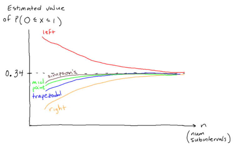
PART 2¶

Location: assignment-problems

Skim the following section of http://learnyouahaskell.com/starting-out.

Texas ranges I'm a list comprehension

Create Haskell file ComplicatedList.hs and write a function calcList in that takes an input number n and counts the number of ordered pairs [x,y] that satisfy $-n \leq x,y \leq n$ and $x-y \leq \dfrac{xy}{2} \leq x+y$ and $x,y \notin \{ -2, -1, 0, 1, 2 \}.$ This function should generate a list comprehension and then count the length of that list.

To check your function, print calcList 50. You should get a result of $16.$

PART 3¶

Complete these C++/Shell/SQL coding challenges and submit screenshots.

https://www.hackerrank.com/challenges/c-tutorial-for-loop/problem

https://www.hackerrank.com/challenges/c-tutorial-functions/problem

https://www.hackerrank.com/challenges/bash-tutorials---comparing-numbers/problem

https://www.hackerrank.com/challenges/bash-tutorials---more-on-conditionals/problem

https://sqlzoo.net/wiki/SELECT_within_SELECT_Tutorial (queries 4,5,6)

For C++/Shell, each screenshot should include your username, the problem title, and the "Status: Accepted" indicator.
For SQL, each screenshot should include the problem number, the successful smiley face, and your query.

Here's a helpful example of some bash syntax. (The spaces on the inside of the brackets are really important! It won't work if you remove the spaces, i.e. [$n -gt 100])

read n
if [ $n -gt 100 ] || [ $n -lt -100 ]
then
  echo What a large number.
else
  echo The number is smol.
  if [ $n -eq 13 ]
  then
      echo And it\'s unlucky!!!
  fi
fi

PART 4¶

a.

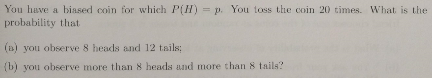
b.

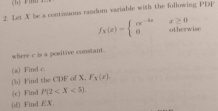
Remember that for a probability distribution $f(x),$ the cumulative distribution function (CDF) is $F(x) = P(X \leq x) = \displaystyle \int_{-\infty}^x f(x) \, \textrm dx.$
Remember that $EX$ means $\textrm E[X].$

Problem 45-3¶

Review; 10% of assignment grade; 15 minutes estimate

Commit your code to GitHub. When you submit your assignment, include a link to your commit(s). If you don't do this, your assignment will receive a grade of $0$ until you resubmit with links to your commits.

Additionally, do the following:

Make 2 GitHub issues on your assigned classmate's repository (but NOT assignment-problems). See eurisko.us/resources/#code-reviews to determine your assigned classmate. When you submit your assignment, include the links to the issues you created.
~Resolve an issue that has been made on your own GitHub repository. When you submit your assignment, include a link to the issue you resolved. (If you don't have any issues on any of your repositories, then you don't have to do anything, but state that this is the case when you turn in your assignment.)~ Let's actually hold off on this bit for the next couple weeks, so that we can build up an inventory of issues on our repositories. Then, once we have an inventory of 5-10 issues to choose from each time, we can start resolving them.

SUBMISSION TEMPLATE¶

For your submission, copy and paste your links into the following template:

Breadth-first and depth-first repl.it link: _____
Commit link for graph repo: _____

Repl.it link to Haskell code: _____
Commit link for assignment-problems repo: _____

Link to C++/SQL screenshots (Overleaf or Google Doc): _____

Link to probability solutions (on Overleaf): _____

Issue 1: _____
Issue 2: _____

Problem 44-1¶

Primary problem; 45% of assignment grade; 75 minutes estimate

Location: Overleaf

a. Submit corrections to final (put your corrections in an overleaf doc). I made a final review video that goes through each problem, available here: https://vimeo.com/496684498

For each correction, explain

what misunderstanding you had, and
how you get to the correct result.

Important: The majority of the misunderstandings should NOT be "I ran out of time", and when you explain how to get to the correct result, SHOW ALL WORK.

b. A food manufacturing company is testing out some recipes for roast beef sandwiches and peanut butter sandwiches. They fed sandwiches to several subjects, and the subjects rated the sandwiches.

Slices of Roast Beef | Tablespoons of Peanut Butter | Rating |
--------------------------------------------------------------
         0           |               0              |    1   |
         1           |               0              |    2   |
         2           |               0              |    4   |
         4           |               0              |    8   |
         6           |               0              |    9   |
         0           |               2              |    2   |
         0           |               4              |    5   |
         0           |               6              |    7   |
         0           |               8              |    6   |

(i) Create a file machine-learning/analysis/sandwich_ratings.py where you use your linear regressor to fit the following model:

$$ \text{rating} = \beta_0 + \beta_1 \times (\text{slices beef}) + \beta_2 \times (\text{tbsp peanut butter})$$

State this model in your Overleaf document.

(ii) Use your model to predict the rating of a sandwich with $5$ slices of roast beef and no peanut butter. State the prediction in your Overleaf document.

(iii) Use your model to predict the rating of a sandwich with $5$ slices of roast beef AND $5$ tablespoons of peanut butter (both ingredients on the same sandwich). State the prediction in your Overleaf document.

(iv) Look back at your answers to (ii) and (iii). One of these predictions can be trusted, while the other cannot. Which can be trusted, and why can it be trusted? Which cannot be trusted, and why can't it be trusted? Why is it possible for the model to give a prediction that can't be trusted?

Problem 44-2¶

Supplemental problems; 45% of assignment grade; 75 minutes estimate

PART 1¶

In your machine-learning repository, create a folder machine-learning/datasets/. Go to https://people.sc.fsu.edu/~jburkardt/data/csv/csv.html, download the file airtravel.csv, and put it in your datasets/ folder.

In Python, you can read a csv as follows:

>>> path_to_datasets = '/home/runner/machine-learning/datasets/'
>>> filename = 'airtravel.csv' 
>>> with open(path_to_datasets + filename, "r") as file:
   print(file.read())

"Month", "1958", "1959", "1960"
"JAN",  340,  360,  417
"FEB",  318,  342,  391
"MAR",  362,  406,  419
"APR",  348,  396,  461
"MAY",  363,  420,  472
"JUN",  435,  472,  535
"JUL",  491,  548,  622
"AUG",  505,  559,  606
"SEP",  404,  463,  508
"OCT",  359,  407,  461
"NOV",  310,  362,  390
"DEC",  337,  405,  432

Write a @classmethod called DataFrame.from_csv(path_to_csv, header=True) that constructs a DataFrame from a csv file (similar to how DataFrame.from_array(arr) constructs the DataFrame from an array).

Test your method as follows:

>>> path_to_datasets = '/home/runner/machine-learning/datasets/'
>>> filename = 'airtravel.csv' 
>>> filepath = path_to_datasets + filename
>>> df = DataFrame.from_csv(filepath, header=True)
>>> df.columns
['"Month"', '"1958"', '"1959"', '"1960"']
>>> df.to_array()
[['"JAN"',  '340',  '360',  '417'],
['"FEB"',  '318',  '342',  '391'],
['"MAR"',  '362',  '406',  '419'],
['"APR"',  '348',  '396',  '461'],
['"MAY"',  '363',  '420',  '472'],
['"JUN"',  '435',  '472',  '535'],
['"JUL"',  '491',  '548',  '622'],
['"AUG"',  '505',  '559',  '606'],
['"SEP"',  '404',  '463',  '508'],
['"OCT"',  '359',  '407',  '461'],
['"NOV"',  '310',  '362',  '390'],
['"DEC"',  '337',  '405',  '432']]

PART 2¶

Location: assignment-problems

Skim the following section of http://learnyouahaskell.com/starting-out.

An intro to lists

Create Haskell file ListProcessing.hs and write a function prodFirstLast in Haskell that takes an input list arr and computes the product of the first and last elements of the list. Then, apply this function to the input [4,2,8,5].

Tip: use the !! operator and the length function.

Your file will look like this:

prodFirstLast arr = (your code here)
main = print (prodFirstLast [4,2,8,5])

Note that, to print out an integer, we use print instead of putStrLn.

(You can also use print for most strings. The difference is that putStrLn can show non-ASCII characters like "я" whereas print cannot.)

Run your function and make sure it gives the desired output (which is 20).

PART 3¶

a. Complete these introductory C++ coding challenges and submit screenshots:

https://www.hackerrank.com/challenges/c-tutorial-basic-data-types/problem

https://www.hackerrank.com/challenges/c-tutorial-conditional-if-else/problem

b. Complete these Bash coding challenges and submit screenshots:

https://www.hackerrank.com/challenges/bash-tutorials---a-personalized-echo/problem

https://www.hackerrank.com/challenges/bash-tutorials---the-world-of-numbers/problem

(Each screenshot should include your username, the problem title, and the "Status: Accepted" indicator.)

c. Complete SQL queries 1-3 here and submit screenshots:

https://sqlzoo.net/wiki/SELECT_within_SELECT_Tutorial

(Each screenshot should include the problem number, the successful smiley face, and your query.)

PART 4¶

a. As we will see in the near future, the standard normal distribution comes up A LOT in the context of statistics. It is defined as

$$ p(x) = \dfrac{1}{\sqrt{2\pi}} e^{-x^2/2}. $$

The reason why we haven't encountered it until now is that it's difficult to integrate. In practice, it's common to use a pre-computed table of values to look up probabilities from this distribution.

The actual problem: Write a function calc_standard_normal_probability(a,b) to approximate $P(a \leq X \leq b)$ for the standard normal distribution, using a Riemann sum with step size 0.001.

To check your function, print out estimates of the following probabilities:

$P(-1 \leq x \leq 1)$
$P(-2 \leq x \leq 2)$
$P(-3 \leq x \leq 3)$

Your estimates should come out close to 0.68, 0.955, 0.997 respectively. (https://en.wikipedia.org/wiki/68%E2%80%9395%E2%80%9399.7_rule)

b.

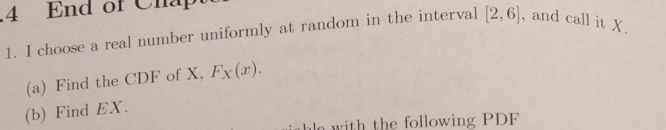
"CDF" stands for Cumulative Distribution Function. The CDF of a probability distribution $f(x)$ is defined as $$ F(x) = P(X \leq x) = \int_{-\infty}^x f(x) \, \textrm dx. $$
Your answer for the CDF will be a piecewise function (3 pieces).
$EX$ means $E[X].$

c.

Problem 44-3¶

Review; 10% of assignment grade; 15 minutes estimate

Commit your code to GitHub. When you submit your assignment, include a link to your commit(s). If you don't do this, your assignment will receive a grade of $0$ until you resubmit with links to your commits.

Additionally, do the following:

Make 2 GitHub issues on your assigned classmate's repository (but NOT assignment-problems). See eurisko.us/resources/#code-reviews to determine your assigned classmate. When you submit your assignment, include the links to the issues you created.
~Resolve an issue that has been made on your own GitHub repository. When you submit your assignment, include a link to the issue you resolved. (If you don't have any issues on any of your repositories, then you don't have to do anything, but state that this is the case when you turn in your assignment.)~ Let's actually hold off on this bit for the next couple weeks, so that we can build up an inventory of issues on our repositories. Then, once we have an inventory of 5-10 issues to choose from each time, we can start resolving them.

Problem 43-1¶

Primary problem; 40% of assignment grade; 60 minutes estimate

In your EulerEstimator, update the plot() method to work with systems of equations. (We wrote this method a while ago, but we've significantly refactored our estimator since then.)

Use the plot() method to plot the system from problem 40-2 on the interval $[0,5],$ using the initial condition $A(0) = B(0) = C(0) = 0$ and step size $\Delta t = 0.01.$

Starting at $t=0,$ step forward with a step size of $\Delta t = 0.01$ until you get to the value $t=5.$
Keep track of the values of the independent variable ($t$) and the dependent variables ($A,B,C$ in this case) as you step forward.
Using the values that you kept track of, plot the curves $y = A(t),$ $y = B(t),$ and $y = C(t)$ on the same graph. Make them different colors.

Once you've got a plot, post it on the #computation-and-modeling channel in Slack to compare with your classmates.

Problem 43-2¶

Supplemental problems; 50% of assignment grade; 75 minutes estimate

PART 1

Location: assignment-problems

Write a function random_draw(distribution) that draws a random number from the probability distribution. Assume that the distribution is an array such that distribution[i] represents the probability of drawing i.

Here are some examples:

random_draw([0.5, 0.5]) will return 0 or 1 with equal probability
random_draw([0.25, 0.25, 0.5]) will return 0 a quarter of the time, 1 a quarter of the time, and 2 half of the time
random_draw([0.05, 0.2, 0.15, 0.3, 0.1, 0.2]) will return 0 5% of the time, 1 20% of the time, 2 15% of the time, 3 30% of the time, 4 10% of the time, and 0.2 20% of the time.

The way to implement this is to

turn the distribution into a cumulative distribution,
choose a random number between 0 and 1, and then
find the index of the first value in the cumulative distribution that is greater than the random number.

Distribution:
    [0.05, 0.2, 0.15, 0.3, 0.1, 0.2]

Cumulative distribution:
    [0.05, 0.25, 0.4, 0.7, 0.8, 1.0]

Choose a random number between 0 and 1:
    0.77431

The first value in the cumulative distribution that is 
greater than 0.77431 is 0.8.

This corresponds to the index 4.

So, return 4.

To test your function, generate 1000 random numbers from each distribution and ensure that their average is close to the true expected value of the distribution.

In other words, for each of the following distributions, print out the true expected value, and then print out the average of 1000 random samples.

[0.5, 0.5]
[0.25, 0.25, 0.5]
[0.05, 0.2, 0.15, 0.3, 0.1, 0.2]

PART 2

Location: assignment-problems

Skim the following sections of http://learnyouahaskell.com/starting-out.

Ready, set, go!
Baby's first functions

Create Haskell file ClassifyNumber.hs and write a function classifyNumber in Haskell that takes an input number x and returns

"negative" if x is negative
"nonnegative" if x is nonnegative.

Then, apply this function to the input 5.

Your file will look like this:

classifyNumber x = (your code here)
main = putStrLn (classifyNumber 5)

Now, run your function by typing the following into the command line:

>>> ghc --make ClassifyNumber
>>> ./ClassifyNumber

ghc is a Haskell compiler. It will compile or "make" an executable object using your .hs file. The command ./ClassifyNumber. actually runs your executable object.

PART 3

Complete this introductory C++ coding challenge: https://www.hackerrank.com/challenges/cpp-input-and-output/problem

Submit a screenshot that includes the name of the problem (top left), your username (top right), and Status: Accepted (bottom).

PART 4

Complete this introductory Shell coding challenge: https://www.hackerrank.com/challenges/bash-tutorials---looping-and-skipping/problem

The following example of a for loop will be helpful:

for i in {2..10}
do
    ((n = 5 * i))
    echo $n
done

Note: You can solve this problem with just a single for loop

Again, submit a screenshot that includes the name of the problem (top left), your username (top right), and Status: Accepted (bottom), just like in part 3.

PART 5

Complete queries 11-14 here: https://sqlzoo.net/wiki/SELECT_from_Nobel_Tutorial

As usual, include a screenshot for each problem that includes the problem number, the successful smiley face, and your query.

PART 6

Location: Overleaf

Complete the following probability problems:

a.

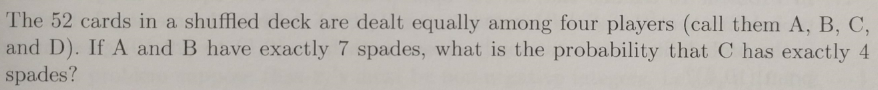
Use conditional probability. In other words, compute the probability that C has exactly $4$ spaces, given that A and B have exactly 7 spaces (together).

b.

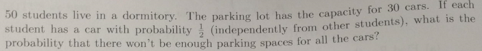
Write your answer using sigma notation or "dot dot dot" notation.

Problem 43-3¶

Review; 10% of assignment grade; 15 minutes estimate

Commit your code to GitHub. When you submit your assignment, include a link to your commit(s). If you don't do this, your assignment will receive a grade of $0$ until you resubmit with links to your commits.

Additionally, do the following:

Make a GitHub issue on your assigned classmate's repository (but NOT assignment-problems). See eurisko.us/resources/#code-reviews to determine your assigned classmate. When you submit your assignment, include a link to the issue you created.
Resolve an issue that has been made on your own GitHub repository. When you submit your assignment, include a link to the issue you resolved. (If you don't have any issues on any of your repositories, then you don't have to do anything, but state that this is the case when you turn in your assignment.)

Problem 42-1¶

Estimated Time: 60 minutes

Grade Weighting: 50%

Complete SQL Zoo Modules 2 (all of it), and problems 1-10 in Module 3 (https://sqlzoo.net/). Put screenshots in an overleaf doc or submit them separately on Canvas (up to you).

Problem 42-2¶

Location: Overleaf

Estimated Time: 45 minutes

Grade Weighting: 50%

Complete the following probability problems, taken from Introduction to Probability: Statistics and Random Processes by Hossein Pishro-Nik:

a.

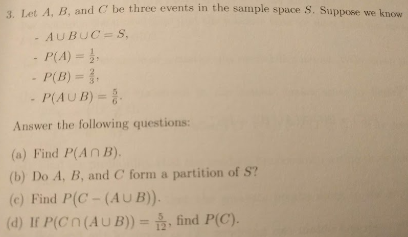
b.

Remember that $\textrm{Var}[A + B] = \textrm{Var}[A] + \textrm{Var}[B] + 2 \textrm{Cov}[A,B].$

c.

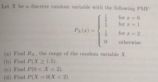
Use Bayes' rule.

d.

Remember that PMF means "probability mass function". This is just the function $P(Z=z).$
Tip: Find the possible values of $Z,$ and then find the probabilities of those values of $Z$ occurring. Your answer will be a piecewise function: $$ P(z) = \begin{cases} \_\_\_, \, z=\_\_\_ \\ \_\_\_, \, z=\_\_\_ \\ \ldots \end{cases} $$

e.

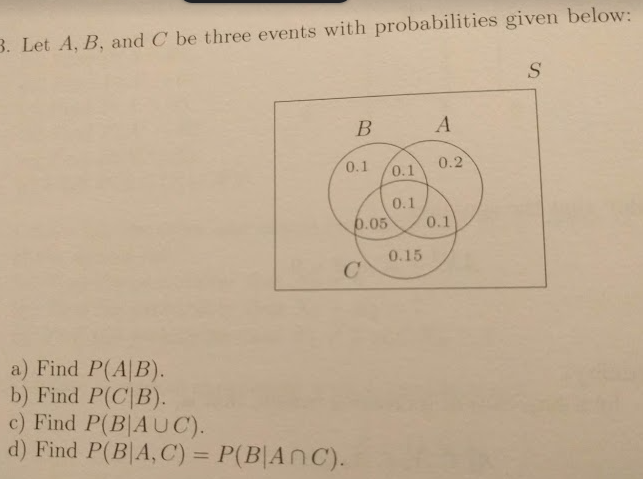
f.

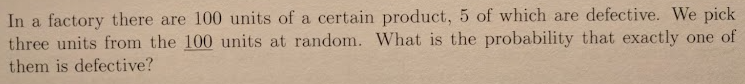
Problem 41-1¶

Wrapping up the semester...

Turn in any missing assignments / resubmissions / quiz corrections by Sunday 1/3 at the very latest. Finish strong! I want to give out strong grades, but I can only do that if you're up to date with all your work and you've done it well.

Problem 41-2¶

Review for the final:

Basic probability

coin flipping, definitions of independent/disjoint, conditional probability, mean, variance, standard deviation, covariance, how variance/covariance are related to expectation

Probability distributions

identifying probability distributions, solving for an unknown constant so that a probability distribution is valid, discrete uniform, continuous uniform, exponential, poisson, using cumulative distributions i.e. P(a <= x < b) = P(x < b) - P(x < a), KL divergence, joint distributions, basic probability computations with joint distributions

Bayesian stats

likelihood distribution, posterior/prior distributions

Regression

pseudoinverse, fitting a linear regression, fitting a logistic regression, end behaviors of linear and logistic regression

Basic algorithms

Basic string processing (something like separate_into_words and reverse_word_order from Quiz 1), Implementing a recursive sequence, euler estimation, unlisting, converting between binary and decimal

Matrix algorithms

matrix multiplication, converting to reduced row echelon form, determinant using rref, determinant using cofactors, why determinant using rref is faster than determinant using cofactors, inverse via augmented matrix

Sorting algorithms

tally sort, merge sort (also know how to merge two sorted lists), swap sort

Optimization algorithms

Newton-Raphson (i.e. the “zero of tangent line” method), gradient descent, grid search (also know how to compute cartesian product)

Data structures

Linked list, tree, stack, queue

Object-oriented programming

Operator overloading, inheritance

Code quality & debugging

Naming conventions, be able to identify good vs bad variable names, be able to identify good vs bad github commits, know how often to make github commits, know the steps for debugging (i.e. print out stuff & use that to figure out where things are going wrong)

Problem 40-1¶

Estimated Time: 30 minutes

Location:

machine-learning/src/linear-regressor.py
machine-learning/tests/test_linear-regressor.py

Grading: 10 points

Extend your LinearRegressor to handle data points of any dimension. Assert that the following tests pass:

>>> df = DataFrame.from_array(
    [[0, 0, 0.1],
     [1, 0, 0.2],
     [0, 2, 0.5],
     [4,5,0.6]],
    columns = ['scoops of chocolate', 'scoops of vanilla', 'taste rating']
)
>>> regressor = LinearRegressor(df, dependent_variable='taste rating')

>>> regressor.coefficients
{
    'constant': 0.19252336,
    'scoops of chocolate': -0.05981308,
    'scoops of vanilla': 0.13271028
}

# these coefficients are rounded, you should only round 
# in your assert statement

>>> regressor.predict({
    'scoops of chocolate': 2,
    'scoops of vanilla': 3
    })
0.47102804

Note: Your class should NOT be tailored to 3-dimensional data points. It should be data points to any number of dimensions.

Problem 40-2¶

Estimated Time: 90 minutes

Location:

simulation/src/euler_estimator.py
simulation/tests/test_euler_estimator.py

Grading: 10 points

Generalize your EulerEstimator to systems of differential equations. For example, we should be able to model the system

$$\begin{align*} A'(t) &= A(t) + 1 \\ B'(t) &= A(t) + B(t) \\ C'(t) &= 2B(t) \end{align*}$$

starting at the point $\left( t, \begin{bmatrix} A \\ B \\ C \end{bmatrix} \right) = \left( 0, \begin{bmatrix} 0 \\ 0 \\ 0 \end{bmatrix} \right)$ as follows:

>>> derivatives = {
        'A': (lambda t,x: x['A'] + 1),
        'B': (lambda t,x: x['A'] + x['B']),
        'C': (lambda t,x: 2*x['B']) 
    }
>>> euler = EulerEstimator(derivatives = derivatives)

>>> initial_values = {'A': 0, 'B': 0, 'C': 0}
>>> initial_point = (0, initial_values)

>>> euler.calc_derivative_at_point(initial_point)
{'A': 1, 'B': 0, 'C': 0}

>>> point_2 = euler.step_forward(point = initial_point, step_size = 0.1)
>>> point_2
(0.1, {'A': 0.1, 'B': 0, 'C': 0})

>>> euler.calc_derivative_at_point(point_2)
{'A': 1.1, 'B': 0.1, 'C': 0}

>>> point_3 = euler.step_forward(point = point_2, step_size = -0.5)
>>> point_3
(-0.4, {'A': -0.45, 'B': -0.05, 'C': 0})

>>> euler.calc_estimated_points(point=point_3, step_size=2, num_steps=3)
[
   (-0.4, {'A': -0.45, 'B': -0.05, 'C': 0}), # starting point 
   (1.6, {'A': 0.65, 'B': -1.05, 'C': -0.2)), # after 1st step
   (3.6, {'A': 3.95, 'B': -1.85, 'C': -4.4)), # after 2nd step
   (5.6, {'A': 13.85, 'B': 2.35, 'C': -11.8)) # after 3rd step
]

Problem 39-1¶

Estimated time: 90 minutes

Grading: 15 points

Location: graph/src/tree.py

In this problem, you will start writing a class Tree that goes in a repository graph. (A tree is a special case of the more general concept of a graph.)

Your Tree class will take in a list of edges, and then the build_from_edges() method will connect up some Nodes with that arrangement of edges. It will be similar to LinkedList, but now a node can have more than one child.

The easiest way to build the tree is as follows:

Look at the edges, identify the root, and create a node for the root.
Look at the edges, identify the children of the root, create a node for each of them, and put that node in the root's children attribute.
For each of those children, identify their children, create a node for each, and put that node in its parent's children attribute.
Keep repeating this procedure until there are no more children to go through

The easiest way is to do a while loop: make a node_array that's initialized as node_array = [self.root], and while node_array is nonempty, do the following:

loop through all nodes in that array, set their children, and put their children in a child_array
Set node_array = list(child_array) .

>>> edges = [('a','c'), ('e','g'), ('e','i'), ('e','a'), ('g','b'), ('a','d'), ('d','f'), ('f','h'), ('d','j'), ('c','k')]
>>> tree = Tree(edges)
>>> tree.build_from_edges()

first, create the root node: e

    e

then, create nodes for the children of e:
    e has children a, i, g

    e
   /|\
  a i g

then, create nodes for the children of a, i, g:
    a has children c, d
    i has no children
    g has a child b

    e
   /|\
  a i g
 /|   |
c d   b

then, create nodes for the children of c, d, b:
    c has a child k
    d has children j and f
    b has no children

    e
   /|\
  a i g
 /|   |
c d   b
| |\
k j f

then, create nodes for the children of k, j, f:
    k has no children
    j has no children
    f has a child h

    e
   /|\
  a i g
 /|   |
c d   b
| |\
k j f
    |
    h

then, create nodes for the children of h:
    h has no children

    e
   /|\
  a i g
 /|   |
c d   b
| |\
k j f
    |
    h

we've run out of children, so we're done

>>> tree.root.value
'e'

>>> [node.value for node in tree.root.children]
['a', 'i', 'g']

# you may need to change the output of this test (and future tests)
# for example, if you have ['g', 'i', 'a'], then that's fine

>>> [node.value for node in tree.root.children[0].children] # children of a
['c', 'd']

# you may need to change the output of this test (and future tests)
# for example, if you had ['g', 'i', 'a'] earlier, then the 
# output would be the children of 'g', which is just ['b']

>>> [node.value for node in tree.root.children[1].children] # children of i
[]

>>> [node.value for node in tree.root.children[2].children] # children of g
['b']

>>> [node.value for node in tree.root.children[0].children[0].children] # children of c
['k']

>>> [node.value for node in tree.root.children[0].children[1].children] # children of d
['j', 'f']

>>> [node.value for node in tree.root.children[2].children[0].children] # children of b
[]

>>> [node.value for node in tree.root.children[0].children[0].children[0].children] # children of k
[]

>>> [node.value for node in tree.root.children[0].children[1].children[0].children] # children of j
[]

>>> [node.value for node in tree.root.children[0].children[1].children[1].children] # children of f
['h']

>>> [node.value for node in tree.root.children[0].children[1].children[1].children[0].children] # children of f
[]

Problem 39-2¶

Estimated Time: 20 min

Location: Overleaf

Grading: 5 points

(Taken from Introduction to Probability: Statistics and Random Processes by Hossein Pishro-Nik)

a.

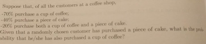
Draw a Venn diagram and use Bayes' Theorem: $P(A \, | \, B) = \dfrac{P(A \textrm{ and } B)}{P(B)}$

b.

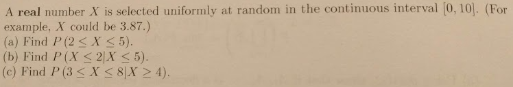
Again, use Bayes' Theorem (but this time, you don't need a Venn diagram).

Problem 38-1¶

Estimated time: 90 minutes

Grading: 15 points

Location: Overleaf

a. Let $X,Y \sim p(x,y).$ Prove that $\textrm{E}[X+Y] = \textrm{E}[X] + \textrm{E}[Y].$

Start with $\textrm{E}[X+Y],$ write the definition in terms of an integral, and then expand out that integral until it can be condensed into $\textrm{E}[X] + \textrm{E}[Y].$

b. The covariance of two random variables $X, Y$ is defined as

$$\text{Cov}[X, Y] = \text{E}[(X - \textrm{E}[X])(Y - \textrm{E}[Y])].$$

Prove that

$$\text{Cov}[X,Y] = \textrm{E}[XY] - \textrm{E}[X] \textrm{E}[Y].$$

It will be fastest to multiply out the product and then expand out the result using part (a).

c. Given that $X \sim U[0,1],$ compute $\text{Cov}[X,X^2].$

It will be fastest to use the identity $\text{Cov}[X,Y] = E[XY] - E[X] E[Y].$
You should get a result of $\dfrac{1}{12}.$

d. Given that $X \sim \mathcal{U}[0,1],$ and $Y \sim \mathcal{U}[0,1],$ we have $(X,Y) \sim \mathcal{U}([0,1] \times [0,1]).$ Compute $\text{Cov}[X, Y].$

It will be fastest to use the identity $\text{Cov}[X,Y] = E[XY] - E[X] E[Y].$
You should get a result of $0.$ (It will always turn out that the covariance of independent random variables is zero.)

e. Prove that

$$\text{Var}[X + Y] = \text{Var}[X] + \text{Var}[Y] + 2 \text{Cov}[X,Y].$$

You can use either of two methods.

Method 1: start with $\textrm{Var}[X+Y],$ write the definition in terms of an integral, and then expand out that integral until it can be condensed the desired result.
Method 2: start with $\textrm{Var}[X+Y],$ then use the identity $\textrm{Var}[A] = \textrm{E}[A^2] - \textrm{E}[A]^2,$ and then use parts (a) and (d).

Problem 38-2¶

Estimated Time: 30 min

Location: Overleaf

Grading: 5 points

Complete Module 8 of Sololearn's C++ Course. Take a screenshot of the completed module, with your user profile showing, and submit it along with the assignment.

Problem 37-1¶

Estimated time: 30 minutes

Grading: 10 points

Location: assignment-problems/tree.py

Write functions get_children, get_parents, and get_roots. Assert that they pass the following tests. Remember that to find the root of the tree, you can just look for the node that has no parents.

>>> edges = [('a','c'), ('e','g'), ('e','i'), ('e','a'), ('d','b'), ('a','d'), ('d','f'), ('f','h'), ('d','j'), ('d','k')]

represents this tree:

    e
   /|\
  a i g
 /|
c d 
 /|\\
b j fk
    |
    h

>>> get_children('e', edges)
['a', 'i', 'g'] # note: the order here doesn't matter -- you can have the
                # children in any order

>>> get_children('c', edges)
[]

>>> get_children('f', edges)
['h']

>>> get_parents('e', edges)
[]

>>> get_parents('c', edges)
['a']

>>> get_parents('f', edges)
['d']

>>> get_roots(edges)
['e']

Problem 37-2¶

Estimated time: 30 minutes

Grading: 10 points

Location: Overleaf

a. Fit a linear regression $y=\beta_0 + \beta_1 x_1 + \beta_2 x_2$ to the following dataset, where points take the form $(x_1, x_2, y).$ This will be the same process as usual, using the pseudoinverse. Show all the steps in your work.

points = [(0, 0, 0.1), (1, 0, 0.2), (0, 2, 0.5), (4,5,0.6)]

b. Fit a logistic regression $y=\dfrac{1}{1+e^{\beta_0 + \beta_1 x_1 + \beta_2 x_2} }$ to the same dataset. Again, show all the steps in your work.

Problem 37-3¶

Estimated time: 30 minutes

Grading: 10 points

Location: Overleaf

Consider the joint exponential distribution defined by

$$p(x,y) = \begin{cases} k e^{-2 x - 3 y} & x,y \geq 0 \\ 0 & x<0 \text{ or } y < 0 \end{cases}.$$

a. Find the value of $k$ such that $p(x,y)$ is a valid probability distribution.

b. Given that $(X,Y) \sim p,$ compute $\text{E}[X]$ and $\text{E}[Y].$

c. Given that $(X,Y) \sim p,$ compute $\text{Var}[X]$ and $\text{Var}[Y].$

d. Given that $(X,Y) \sim p,$ compute $P\left( X < 4, \, Y < 5 \right).$ Write your answer in terms of $e,$ in simplest form.

Problem 36-1¶

Estimated time: 45 minutes

Grading: 10 points

Location: Overleaf

Suppose you are a mission control analyst who is looking down at an enemy headquarters through a satellite view, and you want to get an estimate of how many tanks they have. Most of the headquarters is hidden, but you notice that near the entrance, there are four tanks visible, and these tanks are labeled with the numbers $52, 30, 68, 7.$ So, you assume that they have $N$ tanks that they have labeled with numbers from $1$ to $N.$

Your commander asks you for an estimate: with $95\%$ certainty, what's the max number of tanks they have?

In this problem, you'll answer that question using the same process that you used in 35-1 (a,b,f). In your answer, show your work and justify every step of the way.

Problem 36-2¶

Estimated time: 45 minutes

Grading: 10 points

Location: assignment-problems/grid_search.py

Write a function grid_search(objective_function, grid_lines) that takes the Cartesian product of the grid_lines in the search space, evaluates the objective_function at all points of intersection, and returns the point where the objective_function takes the lowest value.

Assert that it passes the following test:

>>> def two_variable_function(x, y):
        return (x-1)**2 + (y-1)**3

>>> x_lines = [0, 0.25, 0.75]
>>> y_lines = [0.9, 1, 1.1, 1.2]
>>> grid_lines = [x_lines, y_lines]
>>> grid_search(two_variable_function, grid_lines)
[0.75, 0.9]

Note: behind the scenes, grid_search is computing all
intersections of x_lines with y_lines to get the following
points:

[0, 0.9], [0, 1], [0, 1.1], [0, 1.2]
[0.25, 0.9], [0.25, 1], [0.25, 1.1], [0.25, 1.2]
[0.75, 0.9], [0.75, 1], [0.75, 1.1], [0.75, 1.2]

Then, it evaluates the function at these points and returns
the point that gave the lowest value.

Problem 35-1¶

Estimated Time: 60 minutes

Locations: Overleaf AND assignment-problems/assignment_35_stats.py

Grading: 10 points

In this problem, you will perform another round of Bayesian inference, but this time on a different distribution. It will be very similar to Problem 27-3.

Your friend is randomly stating positive integers that are less than some upper bound (which your friend knows, but you don't know). The numbers your friend states are as follows:

1, 17, 8, 25, 3

You assume that the numbers come from a discrete uniform distribution $U\left\{1,2,\ldots,k\right\}$ defined as follows:

$$p_k(x) = \begin{cases} \dfrac{1}{k} & x \in \left\{1,2,\ldots,k\right\} \\ 0 & x \not\in \left\{1,2,\ldots,k\right\} \end{cases}$$

a. Compute the likelihood $P(\left\{ 1, 17, 8, 25, 3 \right\} | \, k).$ Remember that the likelihood is just the probability of getting the result $ \left\{ 1, 17, 8, 25, 3 \right\}$ under the assumption that the data was sampled from the distribution $p_k(x).$ Your answer should be a piecewise function expressed in terms of $k\mathbin{:}$

$$P(\left\{ 1, 17, 8, 25, 3 \right\} | \, k) = \begin{cases} \_\_\_ & k \geq \_\_\_ \\ 0 & \textrm{otherwise} \end{cases}$$

Note: To figure out the $k \geq \_\_\_$ part, keep in mind that the data $\left\{ 1, 17, 8, 25, 3 \right\}$ is drawn from $\left\{ 1, 2, \ldots, k \right\}.$

b. Compute the posterior distribution by normalizing the likelihood. That is to say, find the constant $c$ such that $$\sum_{k=1}^\infty c \cdot P(\left\{ 1, 17, 8, 25, 3 \right\} | \, k) = 1.$$ Then, the posterior distribution will be $$P(k \, | \left\{ 1, 17, 8, 25, 3 \right\})= c \cdot P(\left\{ 1, 17, 8, 25, 3 \right\} \, | \, k).$$

SUPER IMPORTANT: You won't be able to figure this out analytically (i.e. just using pen and paper). Instead, you should write a Python script in assignment-problems/assignment_35_stats.py to approximate the sum by evaluating it for a very large number of terms. You should use as many terms as you need until the result appears to converge.

c. What is the most probable value of $k?$ You can tell this just by looking at the distribution $P(k \, | \left\{ 1, 17, 8, 25, 3 \right\}),$ but make sure to justify your answer with an explanation.

d. The largest number in the dataset is $25.$ What is the probability that $25$ is actually the upper bound chosen by your friend?

e. What is the probability that the upper bound is less than or equal to $30?$

f. Fill in the blank: you can be $95\%$ sure that the upper bound is less than $\_\_\_.$

SUPER IMPORTANT: You won't be able to figure this out analytically (i.e. just using pen and paper). Instead, you should write another Python function in assignment-problems/assignment_35_stats.py to approximate value of $k$ needed (i.e. the number of terms needed) to have $P(K \leq k \, | \left\{ 1, 17, 8, 25, 3 \right\}) = 0.95.$

Problem 35-2¶

Estimated Time: 30 minutes

Location: Overleaf

Grading: 5 points

A joint distribution is a probability distribution on two or more random variables. To work with joint distributions, you will need to use multi-dimensional integrals.

For example, given a joint distribution $p(x,y),$ the distribution must satisfy

$$ \begin{align*} \displaystyle \int_{-\infty}^\infty \int_{-\infty}^\infty p(x,y) \, \text{d}x \, \text{d}y = 1. \end{align*} $$

The probability that $(X,Y) \in [a,b] \times [c,d]$ is given by

$$ \begin{align*} P((X,Y) \in [a,b] \times [c,d]) = \displaystyle \iint_{[a,b] \times [c,d]} p(x,y) \, \text{d}A, \end{align*} $$

or equivalently,

$$ \begin{align*} P(a < X \leq b, \, c < Y \leq d) = \displaystyle \int_c^d \int_a^b p(x,y) \, \text{d}x \, \text{d}y. \end{align*} $$

The expectations are

$$ \begin{align*} \textrm{E}[X] &= \displaystyle \int_c^d \int_a^b x \cdot p(x,y) \, \text{d}x \, \text{d}y, \\ \textrm{E}[Y] &= \displaystyle \int_c^d \int_a^b y \cdot p(x,y) \, \text{d}x \, \text{d}y. \end{align*} $$

The joint uniform distribution $\mathcal{U}([a,b]\times[c,d])$ is a distribution such that all points $(x,y)$ have equal probability in the region $[a,b]\times[c,d]$ and zero probability elsewhere. So, it takes the form

$$p(x,y) = \begin{cases} k & (x,y) \in [a,b] \times [c,d] \\ 0 & (x,y) \not\in [a,b] \times [c,d] \end{cases}$$

for some constant $k.$

a. Find the value of $k$ such that $p(x,y)$ is a valid probability distribution. Your answer should be in terms of $a,b,c,d.$

b. Given that $(X,Y) \sim p,$ compute $\text{E}[X]$ and $\text{E}[Y].$ You should get $\text{E}[X] = \dfrac{a+b}{2}$ and $\text{E}[Y] = \dfrac{c+d}{2}$

c. Geometrically, $[a,b] \times [c,d]$ represents a rectangle bounded by $x=a,$ $x=b,$ $y=c,$ and $y=d.$ What is the geometric interpretation of the point $(\text{E}[X], \text{E}[Y])$ in this rectangle?

Problem 34-1¶

Location: assignment-problems/cartesian_product.py

Estimated Time: 45 minutes

Grading: 10 points

Write a function cartesian_product(arrays) that computes the Cartesian product of all the lists in arrays.

>>> cartesian_product([['a'], [1,2,3], ['Y','Z']])
[['a',1,'Y'], ['a',1,'Z'], ['a',2,'Y'], ['a',2,'Z'], ['a',3,'Y'], ['a',3,'Z']]

NOTE: This is a reasonably short function if you use the following procedure. You'll probably have to think a bit in order to get the implementation correct, though. (Make sure to post for help if you get stuck!)

Create a variable points that will be a list of all the points in the cartesian product. Initially, set points to consist of a single empty point: points = [[]].
For each array in the input, create a new list of points.
- The new set of points can be constructed by looping through each existing point and, for each existing point, adding several new points.
  - For a given point, the new points can be constructed by appending each element of the array onto a copy of the given point.
Return the list of points.

Worked Example:

arrays = [['a'], [1,2,3], ['Y','Z']]

points: [[]]
considering array ['a']
considering element 'a'
new point ['a']

points: [['a']]
considering array [1,2,3]
considering element 1
new point ['a',1]
considering element 2
new point ['a',2]
considering element 3
new point ['a',3]

points: [['a',1], ['a',2], ['a',3]]
considering array ['Y','Z']
considering element 'Y'
new points ['a',1,'Y'], ['a',2,'Y'], ['a',3,'Y']
considering element 'Z'
new points ['a',1,'Z'], ['a',2,'Z'], ['a',3,'Z']

points: [[1,'a','Y'], [1,'a','Z'], [1,'b','Y'], [1,'b','Z'], [1,'c','Y'], [1,'c','Z']]

Watch out! If you write new_point = old_point, then this just makes it so that new_point refers to old_point. So then whenever you change one of those variables, the other will change as well.

To actually make a separate independent copy, you can use new_point = list(old_point). That way, when you change one of the variables, it will have no effect on the other.

Problem 34-2¶

Locations:

machine-learning/src/gradient_descent.py
machine-learning/tests/test_gradient_descent.py

Estimated Time: 60 minutes

Grading: 10 points

Write a class GradientDescent that performs gradient descent on an input function with any number of arguments. This builds on top of Problem 25-1.

Tip: if you have a function f(x,y,z) and a list args = [0,5,3], then you can pass f(*args) to evaluate f(0,5,3).**
Tip: to get the number of variables that a function accepts as input, use f.__code__.co_argcount. For example:
```
>>> def f(x,y): return x**2 + y**2
>>> f.__code__.co_argcount
2
```

Assert that your GradientDescent passses the following tests. (Make sure to post for help if you get stuck!)

Note: the tests below are shown rounded to 3 decimal places. You should do the rounding in your assert statement, NOT in your GradientDescent class.

>>> def single_variable_function(x):
        return (x-1)**2
>>> def two_variable_function(x, y):
        return (x-1)**2 + (y-1)**3
>>> def three_variable_function(x, y, z):
        return (x-1)**2 + (y-1)**3 + (z-1)**4
>>> def six_variable_function(x1, x2, x3, x4, x5, x6):
        return (x1-1)**2 + (x2-1)**3 + (x3-1)**4 + x4 + 2*x5 + 3*x6

>>> minimizer = GradientDescent(f=single_variable_function, initial_point=[0])
>>> minimizer.point
[0]
>>> ans = minimizer.compute_gradient(delta=0.01)
[-2.000] # rounded to 5 decimal places
>>> minimizer.descend(alpha=0.001, delta=0.01, num_steps=1)
>>> minimizer.point
[0.002]

>>> minimizer = GradientDescent(f=two_variable_function, initial_point=[0,0])
>>> minimizer.point
[0,0]
>>> minimizer.compute_gradient(delta=0.01)
[-2.000, 3.000]
>>> minimizer.descend(alpha=0.001, delta=0.01, num_steps=1)
>>> minimizer.point
[0.002, -0.003]

>>> minimizer = GradientDescent(f=three_variable_function, initial_point=[0,0,0])
>>> minimizer.point
[0,0,0]
>>> minimizer.compute_gradient(delta=0.01)
[-2.000, 3.000, -4.000]
>>> minimizer.descend(alpha=0.001, delta=0.01, num_steps=1)
>>> minimizer.point
[0.002, -0.003, 0.004]

>>> minimizer = GradientDescent(f=six_variable_function, initial_point=[0,0,0,0,0,0])
>>> minimizer.point
[0,0,0,0,0,0]
>>> minimizer.compute_gradient(delta=0.01)
[-2.000, 3.000, -4.000, 1.000, 2.000, 3.000]
>>> minimizer.descend(alpha=0.001, delta=0.01, num_steps=1)
>>> minimizer.point
[0.002, -0.003, 0.004, -0.001, -0.002, -0.003]

Make sure to push your finished code to Github with a commit message that says what you added/changed (you should always commit your code to Github after an assignment).

Problem 34-3¶

Estimated Time: 60 min

Location: Overleaf

Grading: 10 points

Complete Module 7 of Sololearn's C++ Course. Take screenshots of the completed modules, with your user profile showing, and submit them along with the assignment.
Complete queries 1-15 in Module 1 of the SQL Zoo. Here's a reference for the LIKE operator, which will come in handy.

Take a screenshot of each successful query and put them in an overleaf doc. When a query is successful, you'll see a smiley face appear. Your screenshots should look like this:

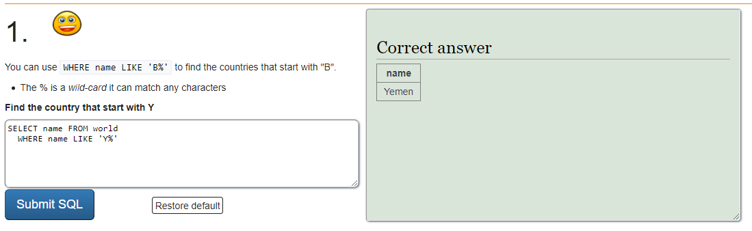
Problem 34-4¶

Take a look at all your assignments so far in this course. If there are any assignments with low grades, that you haven't already resubmitted, then be sure to resubmit them.

Also, if you haven't already, submit quiz corrections for all of the quizzes we've had so far!

Problem 33-1¶

Location: Overleaf

Estimated Time: 60 minutes

Grading: 10 points

Suppose you are again given the following dataset:

data = [(1,0.2), (2,0.25), (3,0.5)]

Fit a logistic regression model $y=\dfrac{1}{1+e^{ax+b}}$ by hand.

Re-express the model in the form $ax+b = \text{some function of }y$ (i.e. isolate $ax+b$ in the logistic regression model). Hint: your function of $y$ will involve $\ln.$
Set up a system of equations and turn the system into a matrix equation.
Find the best approximation to the solution of that matrix equation by using the pseudoinverse.
Substituting your solution for the coefficients of the model, and plot the model along with the 3 given data points on the same graph to ensure that the model fits the data points well.

Show all of your steps. No code allowed in steps 1, 2, and 3! But in step 4, you can write a Python script for the final plot (or make the plot in latex).

Note: To plot points on a graph in Python, you can use the following:

plt.plot([1, 2, 3, 4], [1, 4, 9, 16]) # plot line segments
plt.plot([1, 2, 3, 4], [1, 4, 9, 16], 'ro') # plot red ('r') circles ('o')

import matplotlib.pyplot as plt
plt.plot([1, 2, 3, 4], [1, 4, 9, 16], 'ro') # plot red ('r') circles ('o')

[<matplotlib.lines.Line2D at 0x7fb8ca5bf438>]

Problem 33-2¶

Location: Overleaf

Estimated Time: 30 minutes

Grading: 6 points

a. (2 points) Given that $X \sim p(x),$ where $p(x)$ is a continuous distribution, prove that for any real number $a$ we have $E[aX] = aE[X].$

You should start by writing $E[aX]$ as an integral, manipulating it, and then simplifying the result into $aE[X].$ The manipulation will just be 1 step.

b. (4 points) Given that $X \sim p(x)$ where $p(x)$ is a continuous probability distribution, prove the identity $\text{Var}[X] = E[X^2] - E[X]^2.$

Problem 33-3¶

Estimated Time: 15 min

Grading: 4 points

Complete Module 6 of Sololearn's C++ Course. Take a screenshot of the completed module, with your user profile showing, and submit it along with the assignment.

Problem 32-1¶

Estimated time: 60 min

Grading: 15 points

Locations:

machine-learning/src/linear_regressor.py
machine-learning/tests/test_linear_regressor.py

Create a class LinearRegressor that works as follows. Make sure your code is general. In other words, do not assume the dataset always consists of 3 points, do not assume the independent variable is always named 'progress', etc.

>>> df = DataFrame.from_array(
    [[1,0.2],
     [2,0.25],
     [3,0.5]],
    columns = ['hours worked', 'progress']
)
>>> regressor = LinearRegressor(df, dependent_variable='progress')
>>> regressor.coefficients
[0.01667, 0.15] # meaning that the model is progress = 0.01667 + 0.15 * (hours worked)
# these coefficients are rounded, but you should not round except for
# in your assert statement

>>> regressor.predict({'hours worked': 4})
0.61667

Problem 32-2¶

Estimated Time: 15 min

Grading: 5 points

(Taken from Introduction to Probability: Statistics and Random Processes by Hossein Pishro-Nik)

a.

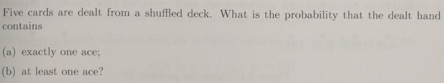
Tip: for (b), compute $1-P(\textrm{complement}).$ Here, the complement is the event that you get no aces.

b.

Tip: again, compute $1-P(\textrm{complement}).$

Problem 32-3¶

Estimated Time: 30 min

Grading: 10 points

Complete Module 5 of Sololearn's C++ Course. Take a screenshot of each completed module, with your user profile showing, and submit both screenshots along with the assignment.
Complete Module 4 of Sololearn's SQL Course. Take a screenshot of the completed module, with your user profile showing, and submit it along with the assignment.

Problem 31-1¶

Estimated Time: 60 min

Grading: 20 points

a.

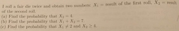
Just count up the number of outcomes in favor, and divide by the total number of possible outcomes

b.

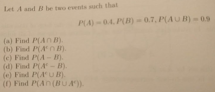
Here is a link to a similar problem, worked out.
Remember that $A^C$ is the "complement" of $A,$ meaning all the space that is NOT included in $A.$
Remember that $A - B = \{ a \in A \, | \, a \not \in B \}.$ For example, $\{ 1, 2, 3 \} - \{2, 4, 6 \} = \{ 1, 3 \}.$

c.

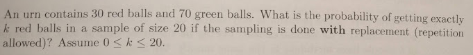
"With replacement" means that each time a ball is drawn, it is put back in for the next draw. So, it would be possible to draw the same ball more than once.
Multiply the following: (number of ways to choose k red balls in a sample of 20) $\times$ (probability of getting k red balls in a row) $\times$ (probability of getting 20-k green balls in a row)
This is very similar to flipping a biased coin, if you think of "red ball" as "heads" and "green ball" as "tails": (number of ways to get k heads in 20 flips) $\times$ (probability of getting k heads in a row) $\times$ (probability of getting 20-k tails in a row)

d.

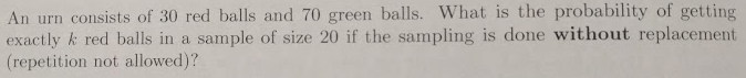
"Without replacement" means that each time a ball is drawn, it is NOT put back in for the next draw. So, it would NOT be possible to draw the same ball more than once.
It's easiest to do this problem if you think of just counting up the number of possibilities in favor, and dividing by the total number of possibilities.
- Possibilities in favor: (number of ways to choose k of the 30 red balls) $\times$ (number of ways to choose 20-k of the 70 green balls)
- Total number of possibilities: (number of ways to choose 20 of the 100 balls)

e.

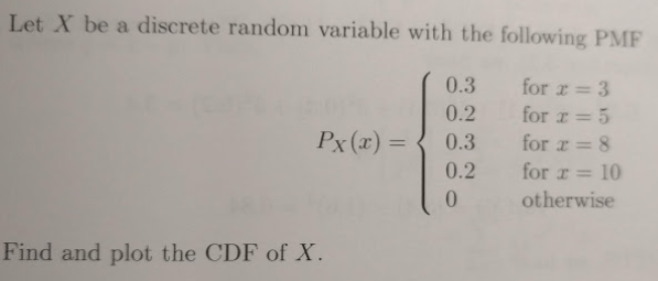
CDF stands for "Cumulative Distribution Function" and is defined as $\textrm{CDF}(x) = P(X \leq x).$
For example, $\textrm{CDF}(6) = P(X \leq 6) = 0.3 + 0.2 = 0.5.$
You're just plotting the function $y=\textrm{CDF}(x).$ You can just draw a picture and put it in your Overleaf doc as an image.

Problem 31-2¶

Estimated Time: 30 min

Grading: 10 points

Complete Module 4 of Sololearn's C++ Course. Take a screenshot of each completed module, with your user profile showing, and submit both screenshots along with the assignment.
Complete Module 3 of Sololearn's SQL Course. Take a screenshot of the completed module, with your user profile showing, and submit it along with the assignment.

Problem 30-1¶

Grading: 10 points

(Taken from Introduction to Probability: Statistics and Random Processes by Hossein Pishro-Nik)

a.

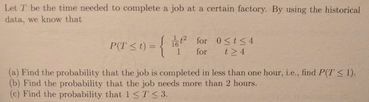
b.

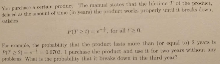
Check: you should get a result of $0.1813.$ If you get stuck, then here's a link to a similar example, worked out.

c.

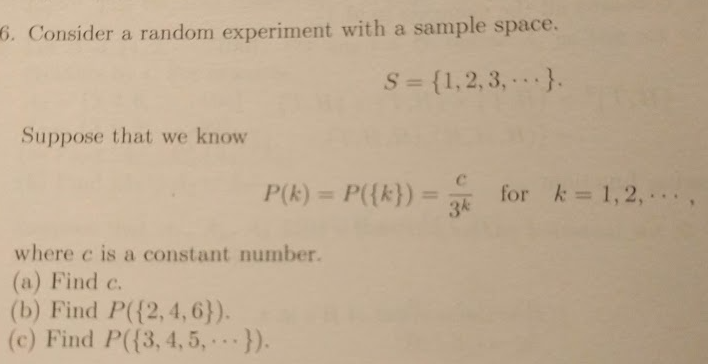
Problem 30-2¶

Location: assignment-problems/doubly_linked_list.py

Grading: 10 points

Create a class DoublyLinkedList that is similar to LinkedList, except that each Node has an additional attribute, prev, which returns the previous node. (It is the opposite of the next attribute.)

Make sure that prev is updated correctly in each of the operations.

Assert that the following test passes:

>>> doubly_linked_list = DoublyLinkedList('a')
>>> doubly_linked_list.append('c')
>>> doubly_linked_list.append('d')
>>> doubly_linked_list.append('e')
>>> doubly_linked_list.insert('b',1)
>>> doubly_linked_list.delete(3)

Note: at this point, the list looks like this:
a <--> b <--> c <--> e

>>> current_node = doubly_linked_list.get_node(3)
>>> node_values = [current_node.data]
>>> for _ in range(3):
        current_node = current_node.prev
        node_values.append(current_node.data)
>>> node_values
['e', 'c', 'b', 'a']

Problem 30-3¶

Grading: 10 points

Complete Module 3 of Sololearn's C++ Course. Take a screenshot of each completed module, with your user profile showing, and submit both screenshots along with the assignment.
Complete Module 2 of Sololearn's SQL Course. Take a screenshot of the completed module, with your user profile showing, and submit it along with the assignment.

Problem 29-1¶

Location: Overleaf

Grading: 10 points

The Poisson distribution can be used to model how many times an event will occur within some continuous interval of time, given that occurrences of an event are independent of one another.

Its probability function is given by \begin{align*} p_\lambda(n) = \dfrac{\lambda^n e^{-\lambda}}{n!}, \quad n \in \left\{ 0, 1, 2, \ldots \right\}, \end{align*}

where $\lambda$ is the mean number of events that occur in the particular time interval.

SUPER IMPORTANT: Manipulating the Poisson distribution involves using infinite sums. However, these sums can be easily expressed using the Maclaurin series for $e^x\mathbin{:}$

\begin{align*} e^x = 1 + x + \dfrac{x^2}{2!} + \dfrac{x^3}{3!} + \ldots \end{align*}

a. Consider the Poisson distribution defined by $$p_2(n) = \dfrac{2^n e^{-2}}{n!}.$$ Show that this is a valid probability distribution, i.e. all the probability sums to $1.$

b. Given that $N \sim p_2,$ compute $P(10 < N \leq 12).$ Leave your answer in exact form, and don't expand out the factorials. Pay close attention to the "less than" vs "less than or equal to" symbols.

c. Given that $N \sim p_2,$ compute $E[N].$

Using the Maclaurin series for $e^x,$ your answer should simplify to $2.$
When doing your series manipulations, don't use sigma notation. Instead, write out the first several terms of the series, followed by "dot dot dot", as shown in the Maclaurin series under the "SUPER IMPORTANT" label.

d. Given that $N \sim p_2,$ compute $\text{Var}[N].$ Using the Maclaurin series for $e^x,$ your answer should come out to a nice clean integer.

Using the Maclaurin series for $e^x,$ your answer should again simplify to $2.$
Again, when doing your series manipulations, don't use sigma notation. Instead, write out the first several terms of the series, followed by "dot dot dot", as shown in the Maclaurin series under the "SUPER IMPORTANT" label.
Tip: try multiplying out the binomial before you expand out the sums. Those 3 sums will be easier to compute, individually $$\begin{align*} e^{-2} \sum_{n=0}^\infty (n-2)^2 \dfrac{2^n}{n!} = e^{-2} \sum_{n=0}^\infty n^2 \cdot \dfrac{2^n}{n!} - e^{-2} \sum_{n=0}^\infty 4n \cdot \dfrac{2^n}{n!} + e^{-2} \sum_{n=0}^\infty 4 \cdot \dfrac{2^n}{n!} \end{align*}$$

Problem 29-2¶

Location: machine-learning/tests/test_data_frame.py

Grading: 10 points

Implement the following functionality in your DataFrame, and assert that these tests pass.

a. Loading an array. You'll need to use @classmethod for this one (read about it here).

>>> columns = ['firstname', 'lastname', 'age']
>>> arr = [['Kevin', 'Fray', 5],
           ['Charles', 'Trapp', 17],
           ['Anna', 'Smith', 13],
           ['Sylvia', 'Mendez', 9]]
>>> df = DataFrame.from_array(arr, columns)

b. Selecting rows which satisfy a particular condition (given as a lambda function)

>>> df.select_rows_where(
    lambda row: len(row['firstname']) >= len(row['lastname'])
                and row['age'] > 10
    ).to_array()
[['Charles', 'Trapp', 17]]

Note: It's true that if you're just working with a plain old array, you can't do stuff like row['firstname']. But we're working with a DataFrame class, which means we've got some creative freedom. You'll have to find way to convert a row array to a row dictionary, behind the scenes. In other words, make a function convert_row_from_array_to_dict that takes a row ['Kevin', 'Fray', 5] and converts it to
```
{
  'firstname': 'Kevin',
  'lastname': 'Fray',
  'age': 5
}
```
before you apply the lambda function.

c. Ordering the rows by given column

>>> df.order_by('age', ascending=True).to_array()
[['Kevin', 'Fray', 5],
['Sylvia', 'Mendez', 9],
['Anna', 'Smith', 13],
['Charles', 'Trapp', 17]]

>>> df.order_by('firstname', ascending=False).to_array()
[['Sylvia', 'Mendez', 9],
['Kevin', 'Fray', 5],
['Charles', 'Trapp', 17],
['Anna', 'Smith', 13]]

Problem 29-3¶

Grading: 5 points

Complete Module 1 of Sololearn's SQL Course. Take a screenshot of the completed module, with your user profile showing, and submit it along with the assignment.

Problem 28-1¶

Location: Overleaf

Grading: 10 points

Suppose you are given the following dataset:

data = [(1,0.2), (2,0.25), (3,0.5)]

Fit a linear regression model $y=a+bx$ by hand by

setting up a system of equations,
turning the system into a matrix equation,
finding the best approximation to the solution of that matrix equation by using the pseudoinverse, and
substituting your solution for the coefficients of the model.

Show all of your steps. No code allowed!

Problem 28-2¶

Grading: 5 points

Create an apply method in your DataFrame, that passes the following test:

>>> data_dict = {
    'Pete': [1, 0, 1, 0],
    'John': [2, 1, 0, 2],
    'Sarah': [3, 1, 4, 0]
}

>>> df1 = DataFrame(data_dict, column_order = ['Pete', 'John', 'Sarah'])
>>> df2 = df1.apply('John', lambda x: 7 * x)
>>> df2.data_dict
{
    'Pete': [1, 0, 1, 0],
    'John': [14, 7, 0, 14],
    'Sarah': [3, 1, 4, 0]
}

Problem 28-3¶

Location: Overleaf

Grading: 5 points

If you didn't get 100% on problem 27-3, revise it and submit it again on this assignment. If you already got 100%, then these 5 points are free.

Problem 28-4¶

Grading: 5 points

Complete Module 1 AND Module 2 of Sololearn's C++ Course. Take a screenshot of each completed module, with your user profile showing, and submit both screenshots along with the assignment.

Problem 27-1¶

Grading: 2 points

In your Matrix class, overload __rmul__and __pow__ so that you pass the following tests:

>>> A = Matrix([[1, 1, 0],
                [2, -1, 0],
                [0, 0, 3]])

>>> B = 0.1 * A
>>> B.elements
[[0.1, 0.1, 0],
 [0.2, -0.1, 0],
 [0, 0, 0.3]]

>>> C = A**3
>>> C.elements
[[3, 3, 0],
 [6, -3, 0],
 [0, 0, 27]]

Problem 27-2¶

Grading: 5 points

Update EulerEstimator to make plots:

>>> euler = EulerEstimator(derivative = lambda t: t+1)

>>> euler.plot(point=(-5,10), step_size=0.1, num_steps=100)

for this example, the plot should look like the parabola
y = 0.5x^2 + x + 2.5
on the domain -5 <= x <= 5

Problem 27-3¶

Location: Overleaf

Grading: 10 points

Suppose you toss a coin $10$ times and get the result $\text{HHHHT HHHHH}.$ From this result, you estimate that the coin is biased and generally lands on heads $90\%$ of the time. But how sure can you be? Let's quantify it.

a. Compute the likelihood $P(\text{HHHHT HHHHH}\, | \, k)$ where $P(H)=k.$ Remember that the likelihood is just the probability of getting the result $\text{HHHHT HHHHH}$ under the assumption that $P(H)=k.$ Your answer should be expressed in terms of $k.$

b. The likelihood $P(\text{HHHHT HHHHH} \, | \, k)$ can almost be interpreted as a probability distribution for $k.$ The only problem is that it doesn't integrate to $1.$

Create a probability distribution $P(k \, | \, \text{HHHHT HHHHH})$ that is proportional to the likelihood $P(\text{HHHHT HHHHH} \, | \, k).$ In other words, find the function $P(k)$ such that

$$ P(k \, | \, \text{HHHHT HHHHH}) = c \cdot P(\text{HHHHT HHHHH} \, | \, k) $$

for some constant $c,$ and $\displaystyle \int_0^1 P(k \, | \, \text{HHHHT HHHHH}) = 1.$

Note: the distribution $P(k \, | \, \text{HHHHT HHHHH})$ is called the "posterior" distribution because it represents the probability distribution of $k$ after we have observed the event $\text{HHHHT HHHHH}.$
The probability distribution of $k$ before we observed the event is called the "prior" distribution and in this case was given by $P(k) \sim \mathcal{U}[0,1]$ since we did not know anything about whether or not the coin is biased (or how biased it is).

c. Using the prior distribution $P(k) \sim \mathcal{U}[0,1],$ what was the prior probability that the coin was biased towards heads? In other words, what was $P(k > 0.5)?$

d. Using the posterior distribution $P(k \, | \, \text{HHHHT HHHHH}),$ what was the posterior probability that the coin was biased towards heads? In other words, what is $P(k > 0.5 \, | \, \text{HHHHT HHHHH})?$

e. Compare your answers in parts (c) and (d). Did the probability that the coin was biased towards heads increase or decrease, after observing the sequence of flips? Why does this make intuitive sense?

f. Using the posterior distribution, what is the most probable value of $k?$ In other words, what is value of $k$ at which $P(k \, | \, \text{HHHHT HHHHH})$ reaches a maximum? Show your work using the first or second derivative test.

g. Why does your answer to (f) make sense? What's the intuition here?

h. What is the probability that the bias $k$ lies within $0.05$ of your answer to part (g)? In other words, what is the probability that $0.85 < k < 0.95?$

i. Fill in the blank: you can be $99\%$ sure that $P(H)$ is at least $\_\_\_.$

Here's a bit more context about the whole situation and what we're trying to do by calculating these things:

We're flipping a coin and we don't know if it's biased.
We let k represent the probability of getting heads. Initially we don't know if the coin is biased, so we'll just say that k has equal probability of being anything. It might be 0.5 (unbiased), or it might be 0.1 (tails more often), or it might be 0.9 (heads more often), or anything. So the probability of k, denoted P(k). This is called our "prior" distribution because it represents our belief "prior" to flipping the coin.
After we flip the coin 10 times and get HHHHT HHHHH, we gain information about how biased our coin is. It looks like it's way biased towards heads. So we need to update our probability distribution. We will call the updated distribution P(k | HHHHT HHHHH), which is "the probability of k given that we got the flips HHHHT HHHHH". This is called our "posterior" distribution because it represents our belief "posterior" or "after" flipping the coin.
But how do we actually get the posterior distribution? It turns out that (as we will prove later), the posterior distribution is proportional to the likelihood of observing the data that we did. In other words, posterior = c likelihood, which becomes P(k | HHHHT HHHHH) = c P(HHHHT HHHHH | k).
Now, for any probability calculations involving k, we can get more accurate probability measurements by using the posterior distribution P(k | HHHT HHHHH) instead of the prior distribution P(k).

Problem 27-4¶

Grading: this assignment will not be graded unless you do this problem

When you submit your assignment, include a link to your github so that I can review your code. I'm going to put in grade for code quality. The code quality will be graded again at the end of the semester, so you will have an opportunity fix anything that's costing you points before the end of the semester.

Problem 26-1¶

Grading: 10 points

Note: If you're approaching it the right way, this problem will be really quick (15 minutes or less to do both parts).

a. In your Matrix class, implement a method exponent.

Remember that to take the exponent of a matrix, you need to repeatedly multiply the matrix by itself using matrix multiplication. (Don't just exponentiate each element separately.)

Include the following test in tests/test_matrix.py.

>>> A = Matrix([[1, 1, 0],
                [2, -1, 0],
                [0, 0, 3]])
>>> A.exponent(3).elements
[[3, 3, 0],
 [6, -3, 0],
 [0, 0, 27]]

b. Also, overload the following operators:

+ (__add__) for matrix addition,
- (__sub__) for matrix subtraction,
* (__mul__) for scalar multiplication,
@ (__matmul__) for matrix multiplication,
== (__eq__) for equality

Include the following test in tests/test_matrix.py.

>>> A = Matrix(
    [[1,0,2,0,3],
    [0,4,0,5,0],
    [6,0,7,0,8],
    [-1,-2,-3,-4,-5]]
    )

>>> A_t = A.transpose()
>>> A_t.elements
[[ 1,  0,  6, -1],
 [ 0,  4,  0, -2],
 [ 2,  0,  7, -3],
 [ 0,  5,  0, -4],
 [ 3,  0,  8, -5]]

>>> B = A_t @ A
>>> B.elements
[[38,  2, 47,  4, 56],
 [ 2, 20,  6, 28, 10],
 [47,  6, 62, 12, 77],
 [ 4, 28, 12, 41, 20],
 [56, 10, 77, 20, 98]]

>>> C = B * 0.1
>>> C.elements
[[3.8,  .2, 4.7,  .4, 5.6],
 [ .2, 2.0,  .6, 2.8, 1.0],
 [4.7,  .6, 6.2, 1.2, 7.7],
 [ .4, 2.8, 1.2, 4.1, 2.0],
 [5.6, 1.0, 7.7, 2.0, 9.8]]

>>> D = B - C
>>> D.elements
[[34.2,  1.8, 42.3,  3.6, 50.4]
 [ 1.8, 18. ,  5.4, 25.2,  9. ]
 [42.3,  5.4, 55.8, 10.8, 69.3]
 [ 3.6, 25.2, 10.8, 36.9, 18. ]
 [50.4,  9. , 69.3, 18. , 88.2]]

>>> E = D + C
>>> E.elements
[[38,  2, 47,  4, 56],
 [ 2, 20,  6, 28, 10],
 [47,  6, 62, 12, 77],
 [ 4, 28, 12, 41, 20],
 [56, 10, 77, 20, 98]]

>>> E == B
True

>> E == C
False

Problem 26-2¶

Grading: 10 points

a. Extend your Matrix class to include a method cofactor_method_determinant() that computes the determinant recursively using the cofactor method.

Here is an example of using the cofactor method on a $3 \times 3$ matrix
Here is an example of using the cofactor method on a $4 \times 4$ matrix
Don't cram everything into the method cofactor_method_determinant(). You will need to write at least one helper function (if you think about the cofactor method, you should be able to realize what the helper function would need to do).

b. Ensure that your cofactor_method_determinant() passes the same exact tests that you already have for your determinant().

c. In a file machine-learning/analysis/rref_vs_cofactor_method_determinant.py, create a $10 \times 10$ matrix and compute the determinant using determinant() and then cofactor_method_determinant(). Which one is faster, and why do you think it's faster? Write your answer as a comment in your code.

Problem 26-3¶

Location: Overleaf

Grading: 10 points for correct answers with supporting work

Note: For every question, you need to justify your answer, but you don't have to show every single step your work. For example, if you're computing a probability, it would be sufficient to write down the statement of the probability, the corresponding integral, the antiderivative, and then the answer. For example, if

$$ X \sim p(x) = \dfrac{1}{\pi} x \sin x, \quad 0 \leq x \leq \pi,$$

then to compute $P\left( X > \dfrac{\pi}{2} \right),$ all you would have to write down is

$$\begin{align*} P\left( X > \dfrac{\pi}{2} \right) &= \int_{\pi/2}^\pi \dfrac{1}{\pi} x \sin x \, \textrm dx \\ &= \dfrac{1}{\pi} \left[ \sin x - x \cos x \right]_{\pi/2}^\pi \quad \textrm{(IBP)} \\ &= \dfrac{\pi - 1}{\pi}. \end{align*}$$

Part 1

Suppose that you take a bus to work every day. Bus A arrives at 8am but is $x$ minutes late with $x \sim U(0,20).$ Bus B arrives at 8:10 but with $x \sim U(0,10).$ The bus ride is 20 minutes and you need to arrive at work by 8:30.

Remember that $U(a,b)$ means the uniform distribution on $[a,b].$ See problem 23-2 if you need a refresher on exponential distributions.
Recall the formulas for the mean and variance of uniform distributions: If $X \sim \mathcal{U}(a,b),$ then $\textrm{E}[X] = \dfrac{a+b}{2}$ and $\textrm{Var}(X) = \dfrac{(b-a)^2}{12}.$ You can use these formulas without any further justification.

a. If you take bus A, what time do you expect to arrive at work? Justify your answer.

b. If you take bus B, what time do you expect to arrive at work? Justify your answer.

c. If you take bus A, what is the probability that you will arrive on time to work? Justify your answer.

d. If you take bus B, what is the probability that you will arrive on time to work? Justify your answer.

Part 2

Continuing the scenario above, there is a third option that you can use to get to work: you can jump into a wormhole and (usually) come out almost instantly at the other side. The only issue is that time runs differently inside the wormhole, and while you're probably going to arrive at the other end very quickly, there's a small chance that you could get stuck in there for a really long time.

The number of seconds it takes you to come out the other end of the wormhole follows an exponential distribution $\textrm{Exp}(\lambda = 4).$

See problem 23-2 if you need a refresher on exponential distributions.
Recall the formulas for the mean and variance of exponential distributions: If $X \sim \textrm{Exp}(\lambda),$ then $\textrm{E}[X] = \dfrac{1}{\lambda}$ and $\textrm{Var}(X) = \dfrac{1}{\lambda^2}.$ You can use these formulas without any further justification.

a. How long do you expect it to take you to come out of the wormhole? Justify your answer.

b. What's the probability of taking longer than a second to come out of the wormhole? Justify your answer.

c. Fill in the blank: the probability of coming out of the wormhole within ___ seconds is $99.999\%.$ Justify your answer.

d. Your friend says that you shouldn't use the wormhole because there's always a chance that you might get stuck in it for over a day, and if you use the wormhole often, then that'll probably happen sometime within your lifetime. Is this a reasonable fear? Why or why not? Justify your answer by computing the probability that you'll get stuck in the wormhole for over a day if you use the wormhole $10$ times each day for $80$ years.

Hint: It's easier to start by computing the probability that you won't get stuck in the wormhole for over a day on any given trip through the wormhole, and then use that to compute the probability that you won't get stuck in the wormhole for over a day if you use the wormhole $10$ times each day for $80$ years.

Problem 25-1¶

Location: assignment_problems/gradient_descent.py

Grading: 10 points

Extend your gradient descent function

gradient_descent(f,initial_point,alpha=0.01,delta=0.0001,num_iterations=10000)

to work on 2-variable functions. The initial_point will take the form $(x_0, y_0),$ and you will repeatedly update your guesses as follows:

\begin{align*} x_{n+1} &= x_n - \alpha f_x(x_n, y_n) \\ y_{n+1} &= y_n - \alpha f_y(x_n, y_n) \end{align*}

To estimate the partial derivatives $f_x(x_n,y_n)$ and $f_y(x_n,y_n),$ you will again use a central difference quotient:

\begin{align*} f_x(x_n, y_n) &\approx \dfrac{f(x_n+ 0.5 \, \delta, y_n) - f(x_n- 0.5 \, \delta, y_n)}{\delta} \\ f_y(x_n, y_n) &\approx \dfrac{f(x_n, y_n+ 0.5 \, \delta) - f(x_n, y_n- 0.5 \, \delta)}{\delta} \\ \end{align*}

a. State the minimum of the function $f(x,y)=1+x^2+y^2.$ Put this as a comment in your code. (Don't use gradient descent yet -- you should be able to tell the minimum just by looking at the function.)

b. Use your gradient descent function to minimize $f(x,y)=1+x^2+y^2$ starting with the initial guess $(1,2).$

Be sure to set the num_iterations high enough that you get very close to the actual minimum. Your result should match up with what you said in part (a).

c. Find the minimum of the function $f(x,y)=1+x^2 + 2x +y^2 - 9y$ using algebra. (You should complete the square -- here's a refresher if you need it.) Show the steps of your algebra as a comment in your code.

d. Use your gradient descent function to minimize $f(x,y)=1+x^2 + 2x +y^2 - 9y$ starting with the initial guess $(0,0).$

Again, be sure to set the num_iterations high enough that you get very close to the actual minimum. Your result should match up with what you said in part (c).

Problem 25-2¶

Location: machine-learning/src/dataframe.py

Grading: 10 points

Create a class DataFrame that implements the following tests:

>>> data_dict = {
    'Pete': [1, 0, 1, 0],
    'John': [2, 1, 0, 2],
    'Sarah': [3, 1, 4, 0]
}

>>> df1 = DataFrame(data_dict, column_order = ['Pete', 'John', 'Sarah'])
>>> df1.data_dict
{
    'Pete': [1, 0, 1, 0],
    'John': [2, 1, 0, 2],
    'Sarah': [3, 1, 4, 0]
}

>>> df1.columns
['Pete', 'John', 'Sarah']

>>> df1.to_array()
[[1, 2, 3]
 [0, 1, 1]
 [1, 0, 4]
 [0, 2, 0]]

>>> df2 = df1.select_columns(['Sarah', 'Pete'])
>>> df2.to_array()
[[3, 1],
 [1, 0],
 [4, 1],
 [0, 0]]

>>> df2.columns
['Sarah', 'Pete']

>>> df3 = df1.select_rows([1,3])
>>> df3.to_array()
[[0, 1, 1]
 [0, 2, 0]]

Problem 24-1¶

Grading: 10 points

Locations:

simulation/src/euler_estimator.py
simulation/tests/test_euler_estimator.py

Here's a refresher of Euler estimation from AP Calc BC. Suppose that $x'(t) = t+1,$ and we're starting at a point $(1,4),$ and we want to estimate the value of $x(3)$ using a step size of $\Delta t = 0.5.$

The key idea is that $$ x'(t) \approx \dfrac{\Delta x}{\Delta t} \quad \Rightarrow \quad \Delta x \approx x'(t) \Delta t. $$

Let's carry out the Euler estimation:

We start at the point $(1,4).$ The slope at this point is $x'(1)=2,$ and $t$ is increasing by a step size of $\Delta t = 0.5,$ so $x$ will increase by $$\begin{align*} \Delta x &\approx x'(1) \Delta t \\ &= (2)(0.5) \\ &= 1. \end{align*}$$
Now we're at the point $(1.5,5).$ The slope at this point is $x'(1.5)=2.5,$ and $t$ is increasing by a step size of $\Delta t = 0.5,$ so $x$ will increase by $$\begin{align*} \Delta x &\approx x'(1.5) \Delta t \\ &= (2.5)(0.5) \\ &= 1.25. \end{align*}$$
Now we're at the point $(2,6.25).$ The slope at this point is $x'(2)=3,$ and $t$ is increasing by a step size of $\Delta t = 0.5,$ so $x$ will increase by $$\begin{align*} \Delta x &\approx x'(2) \Delta t \\ &= (3)(0.5) \\ &= 1.5. \end{align*}$$
Now we're at the point $(2.5,7.75).$ The slope at this point is $x'(2.5)=3.5,$ and $t$ is increasing by a step size of $\Delta t = 0.5,$ so $x$ will increase by $$\begin{align*} \Delta x &\approx x'(2.5) \Delta t \\ &= (3.5)(0.5) \\ &= 1.75. \end{align*}$$
Finally, we reach the point $(3,9.5).$ Therefore, we conclude that $x(3) \approx 9.5.$

Here is your task. Create a Github repository simulation and create a file simulation/src/euler_estimator.py that contains a class EulerEstimator. Write this class so that it passes the following tests, which should be placed in simulation/tests/test_euler_estimator.py.

>>> euler = EulerEstimator(derivative = (lambda t: t+1))

>>> euler.calc_derivative_at_point((1,4))
2

>>> euler.step_forward(point=(1,4), step_size=0.5)
(1.5, 5)

>>> euler.calc_estimated_points(point=(1,4), step_size=0.5, num_steps=4)
[
    (1, 4), # starting point
    (1.5, 5), # after 1st step
    (2, 6.25), # after 2nd step
    (2.5, 7.75), # after 3rd step
    (3, 9.5) # after 4th step
]

Problem 24-2¶

Location: Overleaf

Grading: 5 points

Suppose we have a coin that lands on heads with probability $k$ and tails with probability $1-k.$

We flip the coin $5$ times and get $HHTTH.$

a. Compute the likelihood of the observed outcome if the coin were fair (i.e. $k=0.5$). SHOW YOUR WORK!

\begin{align*} P(\text{HHTTH} \, | \, k=0.5) &= P(\text{H}\, | \, k=0.5) \cdot P(\text{H}\, | \, k=0.5) \cdot P(\text{T}\, | \, k=0.5) \cdot P(\text{T}\, | \, k=0.5) \cdot P(\text{H}\, | \, k=0.5) \\ &= \, ? \end{align*}

\begin{align*}
P(\text{HHTTH} \, | \, k=0.5) &= P(\text{H}\, | \, k=0.5) \cdot P(\text{H}\, | \, k=0.5) \cdot P(\text{T}\, | \, k=0.5) \cdot P(\text{T}\, | \, k=0.5) \cdot P(\text{H}\, | \, k=0.5) \\
&= \, ?
\end{align*}

Check: your answer should come out to $0.03125 \, .$

b. Compute the likelihood of the observed outcome if the coin were slightly biased towards heads, say $k=0.55.$ SHOW YOUR WORK!

\begin{align*} P(\text{HHTTH} \, | \, k=0.55) &= P(\text{H}\, | \, k=0.55) \cdot P(\text{H}\, | \, k=0.55) \cdot P(\text{T}\, | \, k=0.55) \cdot P(\text{T}\, | \, k=0.55) \cdot P(\text{H}\, | \, k=0.55) \\ &= \, ? \end{align*}

Check: your answer should round to $0.03369 \, .$

c. Compute the likelihood of the observed outcome for a general value of $p.$ Your answer should be a function of $k.$

\begin{align*} P(\text{HHTTH} \, | \, k) &= P(\text{H}\, | \, k) \cdot P(\text{H}\, | \, k) \cdot P(\text{T}\, | \, k) \cdot P(\text{T}\, | \, k) \cdot P(\text{H}\, | \, k) \\ &= \, ? \end{align*}

Check: When you plug in $k=0.5,$ you should get the answer from part (a), and when you plug in $k=0.55,$ you should get the answer from part (b).

d. Plot a graph of $P(\text{HHTTH} \, | \, k)$ for $0 \leq k \leq 1,$ and include the graph in your writeup. (The template includes an example of how to insert an image into a latex document.)

For your plot, you can either use tikzpicture as shown in the template, or you can create a Python plot and insert it as a png.

Problem 23-1¶

Implement the algorithm merge_sort that you carried by hand in Assignment 22. Make sure to follow the pseudocode that was provided. Assert that your function passes the following test:

>>> merge_sort([4,8,7,7,4,2,3,1])
[1,2,3,4,4,7,7,8]

Problem 23-2¶

Location: Overleaf

Grading: 8 points

Note: Points will be deducted for poor latex quality. If you're writing up your latex and anything looks off, make sure to post about it so you can fix it before you submit. FOLLOW THE LATEX COMMANDMENTS!

PART 1

Consider the general exponential distribution defined by $$p_\lambda(x) = \begin{cases} \lambda e^{-\lambda x} & x \geq 0 \\ 0 & x < 0 \end{cases}.$$

a. Using integration, show that this is a valid distribution, i.e. all the probability integrates to $1.$

b. Given that $X \sim p_\lambda,$ compute $P(0 < X < 1).$

c. Given that $X \sim p_\lambda,$ compute $\mathrm{E}[X].$

d. Given that $X \sim p_\lambda,$ compute $\text{Var}[X].$

Note: Your answers should match those from Assignment 20 when you substitute $\lambda = 2.$

PART 2

Consider the general uniform distribution on the interval $[a,b].$ It takes the following form for some constant $k\mathbin{:}$

$$p(x) = \begin{cases} k & x \in [a,b] \\ 0 & x \not\in [a,b] \end{cases}$$

a) Find the value of $k$ such that $p(x)$ is a valid probability distribution. Your answer should be in terms of $a$ and $b.$

b) Given that $X \sim p,$ compute the cumulative distribution $P(X \leq x).$ Your answer should be a piecewise function:

$$P(X \leq x) = \begin{cases} \_\_\_ &\text{ if } x < a \\ \_\_\_ &\text{ if } a \leq x \leq b \\ \_\_\_ &\text{ if } b < x \end{cases}$$

c) Given that $X \sim p,$ compute $\mathrm{E}[X].$

d) Given that $X \sim p,$ compute $\text{Var}[X].$

Note: Your answers should match those from Assignment 21 when you substitute $a = 3, b=7.$

Problem 22-1¶

Location: assignment_problems/gradient_descent.py

Grading: 10 points

Write a function gradient_descent(f,x0,alpha=0.01,delta=0.0001,iterations=10000) that uses gradient descent to estimate the minimum of $f(x),$ given the initial guess $x=x_0.$ Here's a visualization of how it works.

The gradient descent algorithm involves repeatedly updating the guess by moving slightly down the slope of the function:

$$x_{n+1} = x_n - \alpha f'(x_n),$$

where $\alpha$ (alpha) is a constant called the learning rate.

Like before, you should estimate $f'(x_n)$ using a central difference quotient,

$$f'(x_n) \approx \dfrac{f(x_n+0.5 \, \delta) - f(x_n- 0.5 \, \delta)}{\delta},$$

where $\delta$ (delta) is chosen as a very small constant. (For our cases, $\delta = 0.001$ should be sufficiently small.)

You should stop updating the guess after iterations=10000 times through the updating process.

a. Test gradient_descent on a simple example: estimate the minimum value of

$$f(x)=x^2+2x+1$$

using the initial guess $x_0 = 0.$ (Note: do not work out the derivative by hand! You should estimate it numerically.)

b. Use gradient_descent to estimate the minimum value of

$$f(x)=\frac{x^{2}+\cos\left(x\right)}{e^{\sin\left(x\right)}}$$

using the initial guess $x_0 = 0.$ (Note: do not work out the derivative by hand! You should estimate it numerically.) Check your answer by plotting the graph on Desmos.

Problem 22-2¶

Here is pseudocode for a sorting algorithm called merge_sort:

merge_sort(input list):
    if the input list consists of more than one element:
        break up the input list into its left and right halves
        sort the left and right halves by recursively calling merge_sort
        merge the two sorted halves
        return the result
    otherwise, if the input list consists of only one element, then it is already sorted,
        and you can just return it.

Here is an example of how merge_sort sorts a list:

input list:[6,9,7,4,2,1,8,5]
break it in half: [6,9,7,4] [2,1,8,5]
use merge_sort recursively to sort the two halves

    input list: [6,9,7,4]
    break it in half: [6,9] [7,4]
    use merge_sort recursively to sort the two halves

        input list: [6,9]
        break it in half: [6] [9]
        the two halves have only one element each, so they are already sorted
        so we can merge them to get [6,9]

        input list: [7,4]
        break it in half: [7] [4]
        the two halves have only one element each, so they are already sorted
        so we can merge them to get [4,7]

    now we have two sorted lists [6,9] and [4,7]
    so we can merge them to get [4,6,7,9]

    input list: [2,1,8,5]
    break it in half: [2,1] [8,5]
    use merge_sort recursively to sort the two halves

        input list: [2,1]
        break it in half: [2] [1]
        the two halves have only one element each, so they are already sorted
        so we can merge them to get [1,2]

        input list: [8,5]
        break it in half: [8] [5]
        the two halves have only one element each, so they are already sorted
        so we can merge them to get [5,8]

    now we have two sorted lists [1,2] and [5,8]
    so we can merge them to get [1,2,5,8]

now we have two sorted lists [4,6,7,9] and [1,2,5,8]
so we can merge them to get [1,2,4,5,6,7,8,9]

Here is your problem: Manually walk through the steps used to sort the list [4,8,7,7,4,2,3,1] using merge_sort. Use the same format as is shown above.

Problem 21-1¶

Location: assignment-problems/merge_sort.py

Grading: 10 points

Write a function merge(x,y) that combines two sorted lists x and y so that the result itself is also sorted. You should run through each list in parallel, keeping track of a separate index in each list, and repeatedly bring a copy of the smallest element into the output list.

>>> merge([-2,1,4,4,4,5,7],[-1,6,6])
[-2,-1,1,4,4,4,5,6,6,7]

Problem 21-2¶

Location: Overleaf

Grading: 10 points

Note: Points will be deducted for poor latex quality. If you're writing up your latex and anything looks off, make sure to post about it so you can fix it before you submit. FOLLOW THE LATEX COMMANDMENTS!

SHOW YOUR WORK!

A uniform distribution on the interval $[3,7]$ is a probability distribution $p(x)$ that takes the following form for some constant $k\mathbin{:}$

$$p(x) = \begin{cases} k & x \in [3,7] \\ 0 & x \not\in [3,7] \end{cases}$$

It is also $\mathcal{U}[3,7].$ So, to say that $X \sim \mathcal{U}[3,7],$ is to say that $X \sim p$ for the function $p$ shown above.

a. Find the value of $k$ such that $p(x)$ is a valid probability distribution. (Remember that for a function to be a valid probability distribution, it must integrate to 1.)

b. Given that $X \sim \mathcal{U}[3,7],$ compute $\text{E}[X].$

Check: does your result make intuitive sense? If you pick a bunch of numbers from the interval $[3,7],$ and all of those numbers are equally likely choices, then what would you expect to be the average of the numbers you pick?

c. Given that $X \sim \mathcal{U}[3,7],$ compute $\text{Var}[X].$

You should get $\dfrac{4}{3}.$

Problem 21-3¶

Grading: 10 points

Extend your Matrix class to include a method determinant() that computes the determinant.

You should do this by copying the same code as in your rref() method, but this time, keep track of the scaling factors by which you divide the rows of the matrix, and keep track of the total number of row swaps.

If the reduced row echelon form DOES NOT come out to the identity, then the determinant is zero.
If the reduced row echelon form DOES come out to the identity, then:
- the magnitude of the determinant is the product of the scaling factors
- the sign of the determinant is $(-1)$ raised to the power of the number of row swaps

Assert that your determinant() method passes the following tests:

>>> A = Matrix(elements = [[1,2]
                           [3,4]])
>>> ans = A.determinant()
>>> round(ans,6)
-2

>>> A = Matrix(elements = [[1,2,0.5]
                           [3,4,-1],
                           [8,7,-2]])
>>> ans = A.determinant()
>>> round(ans,6)
-10.5

>>> A = Matrix(elements = [[1,2,0.5,0,1,0],
                           [3,4,-1,1,0,1],
                           [8,7,-2,1,1,1],
                           [-1,1,0,1,0,1],
                           [0,0.35,0,-5,1,1],
                           [1,1,1,1,1,0]])
>>> ans = A.determinant()
>>> round(ans,6)
-37.3

>>> A = Matrix(elements = [[1,2,0.5,0,1,0],
                           [3,4,-1,1,0,1],
                           [8,7,-2,1,1,1],
                           [-1,1,0,1,0,1],
                           [0,0.35,0,-5,1,1],
                           [1,1,1,1,1,0],
                           [2,3,1.5,1,2,0]])
>>> ans = A.determinant()
Error: cannot take determinant of a non-square matrix

>>> A = Matrix(elements = [[1,2,0.5,0,1,0,1],
                           [3,4,-1,1,0,1,0],
                           [8,7,-2,1,1,1,0],
                           [-1,1,0,1,0,1,0],
                           [0,0.35,0,-5,1,1,0],
                           [1,1,1,1,1,0,0],
                           [2,3,1.5,1,2,0,1]])
>>> ans = A.determinant()
>>> round(ans,6)
0

Problem 20-1¶

Location: Overleaf

Note: Points will be deducted for poor latex quality. If you're writing up your latex and anything looks off, make sure to post about it so you can fix it before you submit. FOLLOW THE LATEX COMMANDMENTS!

Continuous distributions are defined similarly to discrete distributions. There are only 2 big differences:

We use an integral to compute expectation: if $X \sim p,$ then $$E[X] = \int_{-\infty}^\infty x \, p(x) \, \mathrm{d}x.$$
We talk about probability on an interval rather than at a point: if $X \sim p,$ then $$P(a < X \leq b) = \int_a^b p(x) \, \mathrm{d}x$$

Grading: 1 point per correct answer with supporting work

Consider the exponential distribution defined by $$p_2(x) = \begin{cases} 2 e^{-2 x} & x \geq 0 \\ 0 & x < 0 \end{cases}.$$

a. Using integration, show that this is a valid distribution, i.e. all the probability integrates to $1.$

b. Given that $X \sim p_2,$ compute $P(0 < X \leq 1).$

You should get a result of $1-e^{-2}.$

c. Given that $X \sim p_2,$ compute $E[X].$

You should get a result of $\dfrac{1}{2}.$

d. Given that $X \sim p_2,$ compute $\text{Var}[X].$

You should get a result of $\dfrac{1}{4}.$

Problem 20-2¶

Grading: 4 points

Extend your LinkedList to have two additional methods:

delete(index) - delete the node at the given index
insert(new_data, index) - insert a node at the given index, containing the given new_data

>>> linked_list = LinkedList('a')
>>> linked_list.append('b')
>>> linked_list.append('c')
>>> linked_list.append('d')
>>> linked_list.append('e')
>>> linked_list.length()
5
>>> linked_list.print_data()
a
b
c
d
e

>>> linked_list.get_node(2).data
'c'
>>> linked_list.delete(2)
>>> linked_list.length()
4
>>> linked_list.get_node(2).data
'd'
>>> linked_list.print()
a
b
d
e

>>> linked_list.insert('f', 2)
>>> linked_list.length()
5
>>> linked_list.get_node(2).data
'f'
>>> linked_list.print()
a
b
f
d
e

Problem 19-1¶

Location: assignment-problems/zero_of_tangent_line.py

a. (1 point) Write a function estimate_derivative(f, c, delta) that estimates the derivative of the function f(x) at the point x=c using a symmetric difference quotient:

$$ \text{estimate_derivative}(f,c,\delta) = \dfrac{f(c + 0.5 \, \delta) - f(c - 0.5 \, \delta)}{\delta} $$

b. (4 points) Using your function estimate_derivative, generalize your functions zero_of_tangent_line and estimate_solution to work for any input function f(x). They should now have the following inputs:

zero_of_tangent_line(f, c, delta) - compute the zero of the tangent line to the function f(x) at the point x=c, using a symmetric difference quotient with parameter delta
estimate_solution(f, initial_guess, delta, precision) - estimate the zero of f(x) by starting with initial_guess and repeatedly calling zero_of_tangent_line (with parameter delta) until the next guess is within precision of the previous guess.

Note: You should no longer hard-code the derivative. Instead, you'll use estimate_derivative, which should work on any function that is passed in as input.

Assert that your code passes the following tests:

>>> def f(x):
        return x**3 + x - 1

>>> answer = estimate_derivative(f, 0.5, 0.001)
>>> round(answer,6)
1.75

>>> answer = zero_of_tangent_line(f, 0.5, 0.001)
>>> round(answer,6)
0.714286

>>> answer = estimate_solution(f, 0.5, 0.001, 0.01)
>>> round(answer, 6)
0.682328

Problem 19-2¶

Location: Overleaf

Grading: 7 points

To say that a random variable $N$ follows a probability distribution $p(n),$ is to say that $P(N=n) = p(n).$ Symbolically, we write $X \sim p.$

The expected value (also known as the mean) of a random variable $N \sim p$ is defined as the weighted sum of possible values, where the weights are given by the probability.

In other words, $E[N] = \sum n \cdot p(n).$

The variance of a random variable is the expected squared deviation from the mean.

In other words, $\text{Var}[N] = E[(N-E[N])^2]$

Warning: No points will be given if you don't show your work.

PART 1 (1 point per correct answer with supporting work)

a. Write the probability distribution $p_{4}(n)$ for getting $n$ heads on $4$ coin flips, where the coin is a fair coin (i.e. it lands on heads with probability $0.5$).

b. Let $N$ be the number of heads in $4$ coin flips. Then $N \sim p_{4}.$ Intuitively, what is the expected value of $N?$ Explain the reasoning behind your intuition.

c. Compute the expected value of $N,$ using the definition $E[N] = \sum n \cdot p(n).$

The answer you get should match your answer from (b).

d. Compute the variance of $N,$ using the definition $\text{Var}[N] = E[(N-E[N])^2].$

Your answer should come out to $1.$

Part 2 (1 point per correct answer with supporting work)

a. Write the probability distribution $p_{4,k}(n)$ for getting $n$ heads on $4$ coin flips, where the coin is a biased coin that lands on heads with probability $k.$

If you substitute $k=0.5,$ you should get the same result that you did in part 1a.

b. Let $N$ be the number of heads in $4$ coin flips of a biased coin. Then $N\sim p_{4,k}.$ Intuitively, what is the expected value of $N?$ Your answer should be in terms of $k.$ Explain the reasoning behind your intuition.

If you substitute $k=0.5,$ you should get the same result that you did in part 1b.

c. Compute the expected value of $N,$ using the definition $E[N] = \sum n \cdot p(n).$

The answer you get should match your answer from (b).

Problem 18-1¶

Location: assignment-problems/approximations_of_randomness.py

Grading: 5 points

During class, each person created a distribution of coin flips.

flips = {
    'Justin S': 'HTTH HHTT TTHH TTTH HHTH TTHT HHHH THHT THTT HTHH TTTT HTHT TTHH THTH HTTH HHTH HHHT TTTH HTTH HTHT',
    'Nathan R': 'HTTH HHTH HTTT HTHH HTTH HHHH TTHH TTHT THTT HTHT HHTH TTTT THHT HTTH HTHH THHH HTTH THTT HHHT HTHH',
    'Justin H': 'HHHT HHTH HHTT THHT HTTT HTTT HHHT HTTT TTTT HTHT THHH TTHT TTHH HTHT TTTT HHHH THHH THTH HHHH THHT',
    'Nathan A': 'HTTH HHHH THHH TTTH HTTT THTT HTHT THHT HTTH TTTT HHHH TTHH HHTH TTTH HHHH THTT HTHT TTTT HHTT HHTT',
    'Cayden': 'HTHT HHTT HTTH THTH THHT TTHH HHHH TTTH HHHT HTTT TTHT HHTH HTHH THTT HHHH THTT HTTT HTHH TTTT HTTH',
    'Maia': 'HTHH THTH HTTH TTTT TTHT HHHH HHTT THHH TTHH HHTH THHT HHHH THTT HHTH HTHT TTHH TTHH HHHH TTTT HHHT',
    'Spencer': 'HHHT HTTH HTTT HTHH THTT TTHT TTTT HTTH HHTH TTHT TTHH HTHT THHT TTHT THTT THTH HTTH THHT TTTH HHHH',
    'Charlie': 'HHHH HHHT HHTT HTTT TTTT TTTH TTHH THHH THTH HTHT HHTH HTHH TTHT THTT THTH TTHT HTHT THHT HTTH THTH',
    'Anton': 'HHTH THTH TTTT HTTH THTT TTTH THHH TTHH THHT HHHH TTHT HTTT THTH HHHT HHTH HHHH TTTH HTHT TTTT HHTT',
    'William': 'THTT HHHT HTTH THHT THTH HHHT TTTH HHTH THTH HTHT HHHT TTHT HHHT THTT HHTT TTHH HHTH TTTT THTH TTHT'
}

a. Treating these coin flips as simulations of 20 samples of 4 flips, compute the KL divergence between each simulation and the true distribution. Print out your results sorted from "best approximation of randomness" to "worst approximation of randomness".

b. Whose coin flips were the best approximation of truly random coin flips?

Problem 18-2¶

Grading: 5 points

Extend your class Node class to have an additional attribute index that is set by the LinkedList. The head node in the LinkedList will have index 0, the next node will have index 1, and so on.

Extend your class LinkedList to have the following methods:

push(new_data) - insert a new node at the head of the linked list, containing the new_data
get_node(index) - get the node at index

>>> linked_list = LinkedList('b')
>>> linked_list.append('e')
>>> linked_list.append('f')
>>> linked_list.push('a')
>>> linked_list.length()
4

>>> linked_list.head.index
0
>>> linked_list.head.next.index
1
>>> linked_list.head.next.next.index
2
>>> linked_list.head.next.next.next.index
3

>>> linked_list.get_node(0).data
'a'
>>> linked_list.get_node(1).data
'b'
>>> linked_list.get_node(2).data
'e'
>>> linked_list.get_node(3).data
'f'

Problem 17-1¶

Location: assignment-problems/zero_of_tangent_line.py

Notice that we can approximate a zero of a function by repeatedly computing the zero of the tangent line:

a. (2 points) Create a function zero_of_tangent_line(c) that computes the zero of the tangent line to the function $f(x)=x^3+x-1$ at the point $x=c.$

Assert that your code passes the following test:

>>> answer = zero_of_tangent_line(0.5)
>>> round(answer,6)
0.714286

b. (2 points) Create a function estimate_solution(initial_guess, precision) that estimates the solution to $f(x) = x^3+x-1$ by starting with initial_guess and repeatedly calling zero_of_tangent_line until the next guess is within precision of the previous guess.

Asser that your code passes the following test:

>>> answer = estimate_solution(0.5, 0.01)
>>> round(answer, 6)
0.682328

Problem 17-2¶

Locations:

machine-learning/src/matrix.py
machine-learning/tests/test_matrix.py

Grading: 4 points

Extend your Matrix class to include a method inverse() that computes the inverse matrix using Gaussian elimination (i.e. your rref method).

You should do the following:

Start with your matrix $A.$
Augment $A$ with the identity matrix, to create a matrix $[A | I].$
Call reduced row echelon form on your augmented matrix. If the matrix is invertible, then you will get a result $[I|A^{-1}].$
Get the inverse $A^{-1}$ from the row-reduced augmented matrix $[I|A^{-1}].$

If the matrix is not invertible, print a message that explains why -- is it be cause it's singular (i.e. square but has linearly dependent rows), or because it's non-square?

Assert that your inverse method passes the following tests:

>>> A = Matrix([[1, 2],
                [3, 4]])
>>> A_inv = A.inverse()
>>> A_inv.elements
[[-2,   1],
 [1.5, -0.5]]

>>> A = Matrix([[1,   2,  3],
                [1,   0, -1],
                [0.5, 0,  0]])
>>> A_inv = A.inverse()
>>> A_inv.elements
[[0,   0,    2],
 [0.5, 1.5, -4],
 [0,  -1,    2]]

>>> A = Matrix([[1, 2, 3, 0],
                [1, 0, 1, 0],
                [0, 1, 0, 0])
>>> A_inv = A.inverse()
Error: cannot invert a non-square matrix

>>> A = Matrix([[1, 2, 3],
                [3, 2, 1],
                [1, 1, 1])
>>> A_inv = A.inverse()
Error: cannot invert a singular matrix

Problem 16-1¶

Location: assignment-problems/count_compression.py

a. (2 points) Write a function count_compression(string) that takes a string and compresses it into a list of tuples, where each tuple indicates the count of times a particular symbol was repeated.

>>> count_compression('aaabbcaaaa')
[('a',3), ('b',2), ('c',1), ('a',4)]
>>> count_compression('22344444')
[('2',2), ('3',1), ('4',5)]

b. (2 points) Write a function count_decompression(compressed_string) that decompresses a compressed string to return the original result.

>>> count_decompression([('a',3), ('b',2), ('c',1), ('a',4)])
'aaabbcaaaa'
>>> count_decompression([('2',2), ('3',1), ('4',5)])
'22344444'

Problem 16-2¶

Location: assignment-problems/linked_list.py

Grading: 6 points

Create a class LinkedList and a class Node which together implement a singly linked list. A singly linked list is just bunch of Nodes connected up in a line.

The class LinkedList should have exactly one attribute:
- head: gives the node at the beginning of the linked list
Each node should have exactly two attributes:
- data: returns the contents of the node
- next: returns the next node
LinkedList should have exactly three methods:
- print_data(): prints the data of the nodes, starting at the head
- length(): returns the number of nodes in the linked list
- append(): appends a new node to the tail of the linked list

Don't use any Python lists, anywhere.

Assert that your Node class passes the following tests:

>>> A = Node(4)
>>> A.data
4
>>> A.next
None
>>> B = Node(8)
>>> A.next = B
>>> A.next.data
8

Assert that your LinkedList class passes the following tests:

>>> linked_list = LinkedList(4)
>>> linked_list.head.data
4
>>> linked_list.append(8)
>>> linked_list.head.next.data
8
>>> linked_list.append(9)
>>> linked_list.print_data()
4
8
9
>>> linked_list.length()
3

Problem 16-3¶

Grading: 5 points

Make sure your rref() method works.

If it already does, then you are done with this problem and you get a free 5 points.
If it doesn't, you need to fix it this weekend. The next assignment will have a problem that builds on it, so if you don't have it working, you're going to start digging yourself into a hole.
- To debug, use the same method I demonstrated in class on Wednesday: print out everything that's going on, and match it up with the log. Take a look at the recording if you need a refresher on how to do this.
- Post on Slack about any issues you have while debugging, that you can't figure out. I'm happy to look at your code if needed, provided that you've already printed everything out and identified where things first start looking different from the log.

Problem 15-1¶

Location: Write your answers in LaTeX on Overleaf.com using this template.

PART A

The following statements are false. For each statement, explain why it is false, and give a concrete counterexample that illustrates that it is false.

(1 point) If you push 3 elements onto the stack, and then pop off 2 elements, you end up with the last element you pushed.
(1 point) If you push 3 elements onto a queue, and then dequeue 2 elements, you end up with the first element you pushed.
(2 points) Swap sort and simple sort both involve repeatedly comparing two elements. For any given list, the number of pairs of elements that need to be compared by each algorithm is exactly the same.

PART B (4 points)

The following statement is true. First, give a concrete example on which the statement holds true. Then, construct a thorough proof.

Say we flip a coin $n$ times. Let $\widehat{P}(x)$ be the probability of getting $x$ heads according to a Monte Carlo simulation with $N$ samples. Then

$$\widehat{P}(0) + \widehat{P}(1) + \widehat{P}(2) + \cdots + \widehat{P}(n) = 1.$$

Problem 15-2¶

Locations:

machine-learning/src/matrix.py
machine-learning/tests/test_matrix.py

Grading: 4 points for each method with tests

In your Matrix class, write methods augment(other_matrix), get_rows(row_nums), and get_columns(col_nums) that satisfy the following tests:

>>> A = Matrix([
    [1, 2,   3,  4],
    [5, 6,   7,  8],
    [9, 10, 11, 12]
])
>>> B = Matrix([
    [13, 14],
    [15, 16],
    [17, 18]
])

>>> A_augmented = A.augment(B)
>>> A_augmented.elements
[
    [1, 2,   3,  4, 13, 14],
    [5, 6,   7,  8, 15, 16],
    [9, 10, 11, 12, 17, 18]
]

>>> rows_02 = A_augmented.get_rows([0, 2])
>>> rows_02.elements
[
    [1, 2,   3,  4, 13, 14],
    [9, 10, 11, 12, 17, 18]
]

>>> cols_0123 = A_augmented.get_columns([0, 1, 2, 3])
>>> cols_0123.elements
[
    [1, 2,   3,  4],
    [5, 6,   7,  8],
    [9, 10, 11, 12]
]

>>> cols_45 = A_augmented.get_columns([4, 5])
>>> cols_45.elements
[
    [13, 14],
    [15, 16],
    [17, 18]
]

Problem 14-1¶

Location: assignment-problems/shapes.py

Grading: 4 points

Write a class Shape with

attributes base, height, and color
methods describe() and render()

Then, rewrite your classes Rectangle and RightTriangle so that they are child classes that inherit from the parent class Shape.

The reason why we might do this is that we'd like to avoid duplicating the describe() and render() methods in each subclass. This way, you'll only have to write the these methods once, in the Shape class.

Problem 14-2¶

Location: assignment-problems/card_sort.py

Grading: 4 points

Write a function card_sort(num_list) that sorts the list num_list from least to greatest by using the method that a person would use to sort cards by hand.

For example, to sort num_list = [12, 11, 13, 5, 6], we would go through the list and repeatedly put the next number we encounter in the appropriate place relative to the numbers that we have already gone through.

starting list: [12, 11, 13, 5, 6]
initialize sorted list: []

first element is 12
put it in the sorted list:
[12]

next element is 11
put it in the sorted list at the appropriate position:
[11, 12]

next element is 13
put it in the sorted list at the appropriate position:
[11, 12, 13]

next element is 5
put it in the sorted list at the appropriate position:
[5, 11, 12, 13]

next element is 6
put it in the sorted list at the appropriate position:
[5, 6, 11, 12, 13]

final sorted list: [5, 6, 11, 12, 13]

Note: You'll have to do a bit of thinking regarding how to put an element in the sorted list at the appropriate position. I'd recommend creating a helper function insert_element_into_sorted_list(element, sorted_list) to do this so that you can solve that problem on its own, and then use that helper function as a part of your main function card_sort.

Tests: Assert that your function card_sort sorts the following lists correctly:

>>> card_sort([12, 11, 13, 5, 6])
[5, 6, 11, 12, 13]

>>> card_sort([5, 7, 3, 5, 1, 3, -1, 1, -3, -1, -3, -1])
[-3, -3, -1, -1, -1, 1, 1, 3, 3, 5, 5, 7]

Problem 13-1¶

Location: assignment-problems/shapes.py

Grading: 4 points

Write a class Square that inherits from Rectangle. Here's an example of how to implement inheritance.

Note: You should not be manually writing any methods in the Square class. The whole point of using inheritance is so that you don't have to duplicate code.

>>> sq = Square(5,'green')
>>> sq.describe()
Base: 5
Height: 5
Color: green
Perimeter: 20
Area: 25
Vertices: [(0,0), (5,0), (5,5), (0,5)]
>>> sq.render()

Problem 13-2¶

Location: assignment-problems/detecting_biased_coins.py

Grading: 4 points

Suppose that you run an experiment where you flip a coin 3 times, and repeat that trial 25 times. You run this experiment on 3 different coins, and get the following results:

coin_1 = ['TTH', 'HHT', 'HTH', 'TTH', 'HTH',
          'TTH', 'TTH', 'TTH', 'THT', 'TTH',
          'HTH', 'HTH', 'TTT', 'HTH', 'HTH',
          'TTH', 'HTH', 'TTT', 'TTT', 'TTT',
          'HTT', 'THT', 'HHT', 'HTH', 'TTH']
coin_2 = ['HTH', 'HTH', 'HTT', 'THH', 'HHH',
          'THH', 'HHH', 'HHH', 'HTT', 'TTH',
          'TTH', 'HHT', 'TTH', 'HTH', 'HHT',
          'THT', 'THH', 'THT', 'TTH', 'TTT',
          'HHT', 'THH', 'THT', 'THT', 'TTT']
coin_3 = ['HHH', 'THT', 'HHT', 'HHT', 'HTH',
          'HHT', 'HHT', 'HHH', 'TTT', 'THH',
          'HHH', 'HHH', 'TTH', 'THH', 'THH',
          'TTH', 'HTT', 'TTH', 'HTT', 'HHT',
          'TTH', 'HTH', 'THT', 'THT', 'HTH']

Let $P_i(x)$ be the experimental probability of getting $x$ heads in a trial of 3 tosses, using the $i$th coin. Plot the distributions $P_1(x),$ $P_2(x),$ and $P_3(x)$ on the same graph. Be sure to label them.

(This is similar to when you plotted the Monte Carlo distributions, but this time you're given the simulation results.)

Based on the plot of the distributions, what conclusions can you make about the coins? For each coin, does it appear to be fair, biased towards heads, or biased towards tails? Write your answer as a comment.

Problem 12-1¶

Location: assignment-problems/tally_sort.py

Grading: 4 points

Write a function tally_sort(num_list) that sorts the list num_list from least to greatest using the following process:

Subtract the minimum from the list so that the minimum is now 0.
Create an array whose indices correspond to the numbers from 0 to the maximum element.
Go through the list num_list and tally up the count for each index.
Transform the tallies into the desired sorted list (with the minimum still equal to 0).
Add the minimum back to get the desired sorted list, with the minimum now equal to the original minimum.

For example, if x = [2, 5, 2, 3, 8, 6, 3], then the process would be as follows:

identify the minimum: 2

subtract off the minimum: [0, 3, 0, 1, 6, 4, 1]

array of tallies: [number of instances of 0, number of instances of 1, number of instances of 2, number of instances of 3, number of instances of 4, number of instances of 5, number of instances of 6]

array of tallies: [0, 0, 0, 0, 0, 0, 0]

loop through the list [0, 3, 0, 1, 6, 4, 1]

first element: 0
increment the array of tallies at index 0
array of tallies: [1, 0, 0, 0, 0, 0, 0]

next element: 3
increment the array of tallies at index 3
array of tallies: [1, 0, 0, 1, 0, 0, 0]

next element: 0
increment the array of tallies at index 0
array of tallies: [2, 0, 0, 1, 0, 0, 0]

next element: 1
increment the array of tallies at index 1
array of tallies: [2, 1, 0, 1, 0, 0, 0]

next element: 6
increment the array of tallies at index 6
array of tallies: [2, 1, 0, 1, 0, 0, 1]

next element: 4
increment the array of tallies at index 4
array of tallies: [2, 1, 0, 1, 1, 0, 1]

next element: 1
increment the array of tallies at index 1
array of tallies: [2, 2, 0, 1, 1, 0, 1]

final array of tallies: [2, 2, 0, 1, 1, 0, 1]

remember what array of tallies represents: [number of instances of 0, number of instances of 1, number of instances of 2, number of instances of 3, number of instances of 4, number of instances of 5, number of instances of 6]

2 instances of 0  --> 0, 0
2 instances of 1  --> 1, 1
0 instances of 2  -->
1 instances of 3  --> 3
1 instances of 4  --> 4
0 instances of 5  -->
1 instances of 6  --> 6

Transform the tallies into the sorted list (with minimum still equal to 0)
[0, 0, 1, 1, 3, 4, 6]

Add the minimum back: [2, 2, 3, 3, 5, 6, 8]

Assert that your function passes the following test:

>>> tally_sort([2, 5, 2, 3, 8, 6, 3])
[2, 2, 3, 3, 5, 6, 8]

Note: Don't use the built-in functions max() nor min(). Rather, if you want to use either of these functions, you should write your own.

Problem 12-2¶

Location: assignment-problems/shapes.py

Grading: 4 points total

Observe the following plotting example:

import matplotlib.pyplot as plt
plt.style.use('bmh')

plt.plot(
    [0, 1, 2, 0],  # X-values
    [0, 1, 0, 0],   # Y-values
    color='blue'
)
plt.gca().set_aspect("equal")
plt.savefig('triangle.png')

a. (2 points)

Write a class Rectangle.

include the attributes base, height, color, perimeter, area, and vertices.
- only base, height, and color should be used as parameters
include a method describe() that prints out the attributes of the rectangle.
include a method render() that renders the rectangle on a cartesian plane. (You can use plt.plot() and plt.gca() and plot.gca().set_aspect("equal") as shown above.)

>>> rect = Rectangle(5,2,'red')
>>> rect.describe()
Base: 5
Height: 2
Color: red
Perimeter: 14
Area: 10
Vertices: [(0,0), (5,0), (5,2), (0,2)]
>>> rect.render()

b. (2 points)

Write a class RightTriangle.

Include the attributes base, height, color, perimeter, area, and vertices.
Include a method describe() that prints out the attributes of the right triangle.
include a method render() that draws the triangle on a cartesian plane.

>>> tri = RightTriangle(5,2,'blue')
>>> tri.describe()
Base: 5
Height: 2
Color: blue
Perimeter: 12.3851648071
Area: 5
Vertices: [(0,0), (5,0), (0,2)]
>>> tri.render()

Problem 11-1¶

Location: assignment-problems/kl_divergence_for_monte_carlo_simulations.py

Grading: 10 points total

The Kullback–Leibler divergence (or relative entropy) between two probability distributions $p(n)$ and $q(n)$ is defined as

\begin{align*} \mathcal{D}(p \, || \, q) = \sum\limits_{n \text{ such that} \\ p(n), q(n) \neq 0} p(n) \ln \left( \dfrac{p(n)}{q(n)} \right) \end{align*}

Intuitively, the divergence measures how "different" the two distributions are.

a. (4 points)

Write a function kl_divergence(p, q) that computes the KL divergence between two probability distributions p and q, represented as arrays. Test your function by asserting that it passes the following test:

>>> p = [0.2, 0.5, 0, 0.3]
>>> q = [0.1, 0.8, 0.1, 0]
>>> kl_divergence(p,q)
-0.09637237851    (in your test, you can round to 6 decimal places)

Note: the computation for the above is
0.2*ln(0.2/0.1) + 0.5*ln(0.5/0.8)

we exclude the terms 0*ln(0/0.1) and 0.3*ln(0.3/0)
because we're only summing over terms where neither
p(n) nor q(n) is equal to 0

b. (4 points)

Compute the KL divergence where p is the Monte Carlo distribution and q is the true distribution for the number of heads in 8 coin tosses, using 1,000 samples in your Monte Carlo simulation (that's the default number from the previous assignment).

Then do the same computation with 100 samples, and then with 10,000 samples. Print out the results for all 3 computations:

>>> python assignment-problems/kl_divergence_for_monte_carlo_simulations.py

Testing KL Divergence... Passed!

Computing KL Divergence for MC Simulations...
100 samples --> KL Divergence = ___
1,000 samples --> KL Divergence = ___
10,000 samples --> KL Divergence = ___

c. (2 points)

In a comment in your code, write down what the general trend is and why:

# As the number of samples increases, the KL divergence approaches __________ because _______________________________.

Problem 11-2¶

Locations:

machine-learning/src/matrix.py
machine-learning/tests/test_matrix.py

Grading: 5 points for each passing test, 10 points code quality (so 20 points total)

MINOR CODE UPDATES BEFORE YOU DO THE ACTUAL PROBLEM:

Before you do this problem, you need to update some of your previous code so that you don't run into any mutation issues where running methods affects the underlying elements.

a. First, update your `copy()` method so that when it creates a copied matrix, it uses a completely separate array of elements (albeit with the same entries). You can do it like this:

def copy(self):
    copied_elements = [[entry for entry in row] for row in self.elements]
    return Matrix(copied_elements)

(The reason why we need to do this is that whenever Python sees any sort of assignment with an existing list, it doesn't actually make a separate copy of the list. It just "points" to the existing list. We want the copied elements to be completely separate from self.elements.)

b. Second, update your helper methods `self.swap_rows()`, `self.normalize_row()`, `self.clear_below()`, and `self.clear_above()` so that they don't affect the original matrix `self`. In these methods, instead of modifying self.elements you should create a copy of self.elements, modify the copy, and then return the matrix whose elements are the copy.

You will need to update your tests to use A = A.swap_rows(), A = A.normalize_row(), A = A.clear_below(), and A = A.clear_above() as follows:

>>> A = Matrix(elements = [[0, 1, 2],
                           [3, 6, 9],
                           [2, 6, 8]])
>>> A.get_pivot_row(0)
1

>>> A = A.swap_rows(0,1)
>>> A.elements
[[3, 6, 9]
 [0, 1, 2]
 [2, 6, 8]]

>>> A = A.normalize_row(0)
>>> A.elements
[[1, 2, 3]
 [0, 1, 2]
 [2, 6, 8]]

>>> A = A.clear_below(0)
>>> A.elements
[[1, 2, 3]
 [0, 1, 2]
 [0, 2, 2]]

>>> A = A.get_pivot_row(1)
1

>>> A = A.normalize_row(1)
>>> A.elements
[[1, 2, 3]
 [0, 1, 2]
 [0, 2, 2]]

>>> A = A.clear_below(1)
>>> A.elements
[[1, 2, 3]
 [0, 1, 2]
 [0, 0, -2]]

>>> A.get_pivot_row(2)
2

>>> A = A.normalize_row(2)
>>> A.elements
[[1, 2, 3]
 [0, 1, 2]
 [0, 0, 1]]

>>> A = A.clear_above(2)
>>> A.elements
[[1, 2, 0]
 [0, 1, 0]
 [0, 0, 1]]

>>> A = A.clear_above(1)
>>> A.elements
[[1, 0, 0]
 [0, 1, 0]
 [0, 0, 1]]

THE ACTUAL PROBLEM:

Extend your Matrix class to include a method rref that converts the matrix to reduced row echelon form. You should use the row reduction algorithm, which goes like this:

create a copy of the original matrix
row_index = 0
for each col_index:
    if a pivot row exists for the col_index:

        if the pivot row is not the current row:
            swap the current row with the pivot row
            # now the current row is actually the pivot row

        normalize the pivot row so that the first nonzero entry is 1
        clear all entries below and above the pivot entry

        row_index += 1

Assert that your method passes the following tests:

>>> A = Matrix([[0, 1, 2],
                [3, 6, 9],
                [2, 6, 8]])
>>> A.rref().elements
[1, 0, 0]
[0, 1, 0]
[0, 0, 1]

>>> B = Matrix([[0, 0, -4, 0],
                [0, 0, 0.3, 0],
                [0, 2, 1, 0]])
>>> A.rref().elements
[0, 1, 0, 0]
[0, 0, 1, 0]
[0, 0, 0, 0]

To help you debug your implementation, here is a walkthrough of the above algorithm on the matrix $\begin{bmatrix} 0 & 1 & 2 \\ 3 & 6 & 9 \\ 2 & 6 & 8 \end{bmatrix}\mathbin{:}$

row_index = 0

looping through columns...

col_index = 0

    current matrix is
    [0,1,2]
    [3,6,9]
    [2,6,8]

    for col_index = 0, the pivot row has index 1
    this is different from row_index = 0, so we need to swap
    swapping, the matrix becomes
    [3,6,9]
    [0,1,2]
    [2,6,8]

    the pivot row now has index 0, same as row_index = 0
    normalizing the pivot row, the matrix becomes
    [1,2,3]
    [0,1,2]
    [2,6,8]

    the pivot entry is the 1 in the (0,0) position (i.e. top-left)
    clearing all entries above and below the pivot entry, the matrix becomes
    [1,2,3]
    [0,1,2]
    [0,2,2]

    row_index += 1
    so now we have row_index = 1

col_index = 1

    current matrix is
    [1,2,3]
    [0,1,2]
    [0,2,2]

    for col_index = 1, the pivot row has index 1, same as row_index=1
    so no swap is needed

    the pivot row is already normalized

    the pivot entry is the 1 in the (1,1) position (i.e. exact middle)
    clearing all entries above and below the pivot entry, the matrix becomes
    [1,0,-1]
    [0,1,2]
    [0,0,-2]

    row_index += 1
    so now we have row_index = 2

col_index = 2

    current matrix is
    [1,0,-1]
    [0,1,2]
    [0,0,-2]

    for col_index = 2, the pivot row has index 2, same as row_index=2
    so no swap is needed

    normalizing the pivot row, the matrix becomes
    [1,0,-1]
    [0,1,2]
    [0,0,1]

    the pivot entry is the 1 in the (2,2) position (i.e. bottom-right)
    clearing all entries above and below the pivot entry, the matrix becomes
    [1,0,0]
    [0,1,0]
    [0,0,1]

    row_index += 1
    so now we have row_index = 3

we've gone through all the columns, so we're done!
the result is
    [1,0,0]
    [0,1,0]
    [0,0,1]

Likewise, here is a walkthrough of the above algorithm on the matrix $\begin{bmatrix} 0 & 0 & -4 & 0 \\ 0 & 0 & 0.3 & 0 \\ 0 & 2 & 1 & 0 \end{bmatrix}\mathbin{:}$

row_index = 0

looping through columns...

col_index = 0

    current matrix is
    [0,0,-4,0]
    [0,0,0.3,0]
    [0,2,1,0]

    for col_index = 0, there is no pivot row
    so we move on

    we still have row_index = 0

col_index = 1

    current matrix is
    [0,0,-4,0]
    [0,0,0.3,0]
    [0,2,1,0]

    for col_index = 1, the pivot row has index 2
    this is different from row_index = 0, so we need to swap
    swapping, the matrix becomes
    [0,2,1,0]
    [0,0,0.3,0]
    [0,0,-4,0]

    the pivot row now has index 0, same as row_index = 0
    normalizing the pivot row, the matrix becomes
    [0,1,0.5,0]
    [0,0,0.3,0]
    [0,0,-4,0]

    the pivot entry is the 1 in the (0,1) position
    all entries above and the pivot entry are already cleared

    row_index += 1
    so now we have row_index = 1

col_index = 2

    current matrix is
    [0,1,0.5,0]
    [0,0,0.3,0]
    [0,0,-4,0]

    for col_index = 2, the pivot row has index 1, same as row_index = 1
    so no swap is needed

    normalizing the pivot row, the matrix becomes
    [0,1,0.5,0]
    [0,0,1,0]
    [0,0,-4,0]

    the pivot entry is the 1 in the (1,2) position
    clearing all entries above and below the pivot entry, the matrix becomes
    [0,1,0,0]
    [0,0,1,0]
    [0,0,0,0]

    row_index += 1
    so now we have row_index = 2 

col_index = 3

    current matrix is
    [0,1,0,0]
    [0,0,1,0]
    [0,0,0,0]

    for col_index = 3, there is no pivot row
    so we move on

    we still have row_index = 2

we've gone through all the columns, so we're done!
the result is
    [0,1,0,0]
    [0,0,1,0]
    [0,0,0,0]

Problem 10-1¶

Location: assignment-problems/distribution_plots.py

Grading: 6 points

Using your function probability(num_heads, num_flips), plot the distribution for the number of heads in 8 coin flips. In other words, plot the curve $y=p(x),$ where $p(x)$ is the probability of getting $x$ heads in $8$ coin flips.

Then, make 5 more plots, each using your function monte_carlo_probability(num_heads, num_flips). Put all your plots on the same graph, label them with a legend to indicate whether each plot is the true distribution or a monte carlo simulation, and save the figure as plot.png.

Legend: True, MC 1, MC 2, MC 3, MC 4, MC 5.

Make the true distribution thick (linewidth=2.5) and the monte carlo distributions thin (linewidth=0.75). A plotting example for 4 coin flips is shown below to assist you.

Note: You will need to modify the plotting example to make it for 8 coin flips instead of 4.
To be clear, you are just making 1 plot. The plot should contain the true distribution (thick line) and 5 Monte Carlo simulation distributions (thin lines).

import matplotlib.pyplot as plt
plt.style.use('bmh')
plt.plot([0,1,2,3,4],[0.1, 0.3, 0.5, 0.1, 0.1],linewidth=2.5)
plt.plot([0,1,2,3,4],[0.3, 0.1, 0.4, 0.2, 0.1],linewidth=0.75)
plt.plot([0,1,2,3,4],[0.2, 0.2, 0.3, 0.3, 0.2],linewidth=0.75)
plt.legend(['True','MC 1','MC 2'])
plt.xlabel('Number of Heads')
plt.ylabel('Probability')
plt.title('True Distribution vs Monte Carlo Simulations for 4 Coin Flips')
plt.savefig('plot.png')

Problem 10-2¶

Locations: assignment-problems/unlist.py

Grading: In each part, you get 1 point for code quality, and 1 point for passing tests (so 4 points total)

a. WITHOUT using recursion, create a function unlist_nonrecursive(x) that removes outer parentheses from a list until either a) the final list consists of multiple elements, or b) no more lists exist.

Assert that your function passes the following tests.

>>> unlist_nonrecursive([[[[1], [2,3], 4]]])
[[1], [2,3], 4]
>>> unlist_nonrecursive([[[[1]]]])
1

b. USING RECURSION, write a function unlist_recursive(x) and assert that it passes the same tests as in part (a).

Problem 9-1¶

Locations: assignment-problems/collatz_iterations.py

The Collatz function is defined as

$$f(n) = \begin{cases} n \, / \, 2 & \text{if } n \text{ is even} \\ 3n+1 & \text{if } n \text{ is odd} \end{cases}$$

The Collatz conjecture is that by repeatedly applying this function to any positive number, the result will eventually reach the cycle

$$1 \to 4 \to 2 \to 1.$$

For example, repeatedly applying the Collatz function to the number $13,$ we have:

$$13 \to 40 \to 20 \to 10 \to 5 \to 16 \to 8 \to 4 \to 2 \to 1$$

a. (1 point for code quality; 1 point for passing the test)

Create a function collatz_iterations(number) that computes the number of iterations of the Collatz function that it takes for the input number to reach $1.$

>>> collatz_iterations(13)
9

b. (1 point)

Write a short script to answer the following question:

Of the numbers from 1 to 1000, which number has the highest number of Collatz iterations?

c. (1 point)

Make a plot where the horizontal axis is the numbers from 1 to 1000 and the vertical axis is the number of Collatz iterations. You can use the sample code below to help you with plotting.

import matplotlib.pyplot as plt
plt.style.use('bmh')
x_coords = [0,1,2,3,4]
y_coords = [5,3,8,5,1]
plt.plot(x_coords, y_coords)
plt.xlabel('X-Axis Label')
plt.ylabel('Y-Axis Label')
plt.title('This is the title of the plot!')
plt.savefig('plot.png')

Problem 9-2¶

This will be a lighter assignment in case you need to catch up with the Matrix class or the Monte Carlo simulations. They need to be working 100%. Make sure that you've caught up, because we will be pressing forward with them on the next few assignments.

Problem 8-1¶

Locations: machine-learning/src/matrix.py and machine-learning/tests/test_matrix.py

Grading: 5 points for code quality; 5.5 points for passing tests (0.5 point per test)

Implement the following helper methods in your matrix class.

get_pivot_row(self, column_index): returns the index of the topmost row that has a nonzero entry in the desired column_index and such that all entries left of column_index are zero. Otherwise, if no row exists, return None.
swap_rows(self, row_index1, row_index2): swap the row at row_index1 with the row at row_index2.
normalize_row(self, row_index): divide the entire row at row_index by the row's first nonzero entry.
clear_below(self, row_index):
- Let $j$ be the column index of the first nonzero entry in the row at row_index.
- Subtract multiples of the row at row_index from the rows below, so that for any row below row_index, the entry at column $j$ is zero.
clear_above(self, row_index):
- Let $j$ be the column index of the first nonzero entry in the row at row_index.
- Subtract multiples of the row at row_index from the rows above, so that for any row above row_index, the entry at column $j$ is zero.

Watch out!

Remember that the first row/column of a matrix has the index 0, not 1.
If row1 is "below" row2 in a matrix, then row1 actually has a higher index than row2. This is because the 0 index corresponds to the very top row.

Assert that the following tests pass.

>>> A = Matrix(elements = [[0, 1, 2],
                           [3, 6, 9],
                           [2, 6, 8]])
>>> A.get_pivot_row(0)
1

>>> A = A.swap_rows(0,1)
>>> A.elements
[[3, 6, 9]
 [0, 1, 2]
 [2, 6, 8]]

>>> A = A.normalize_row(0)
>>> A.elements
[[1, 2, 3]
 [0, 1, 2]
 [2, 6, 8]]

>>> A = A.clear_below(0)
>>> A.elements
[[1, 2, 3]
 [0, 1, 2]
 [0, 2, 2]]

>>> A = A.get_pivot_row(1)
1

>>> A = A.normalize_row(1)
>>> A.elements
[[1, 2, 3]
 [0, 1, 2]
 [0, 2, 2]]

>>> A = A.clear_below(1)
>>> A.elements
[[1, 2, 3]
 [0, 1, 2]
 [0, 0, -2]]

>>> A.get_pivot_row(2)
2

>>> A = A.normalize_row(2)
>>> A.elements
[[1, 2, 3]
 [0, 1, 2]
 [0, 0, 1]]

>>> A = A.clear_above(2)
>>> A.elements
[[1, 2, 0]
 [0, 1, 0]
 [0, 0, 1]]

>>> A = A.clear_above(1)
>>> A.elements
[[1, 0, 0]
 [0, 1, 0]
 [0, 0, 1]]

Make sure that when you run python tests/test_matrix.py, your tests print out (including your tests from last time)

>>> python tests/test_matrix.py
Testing method "copy"...
PASSED

Testing method "add"...
PASSED

Testing method "subtract"...
PASSED

Testing method "scalar_multiply"...
PASSED

Testing method "matrix_multiply"...
PASSED

Testing row reduction on the following matrix:
[[0, 1, 2],
 [3, 6, 9],
 [2, 6, 8]]

- Testing method "get_pivot_row(0)"...
- PASSED

- Testing method "swap_rows(0,1)"...
- PASSED

- Testing method "normalize_row(0)"...
- PASSED

- Testing method "clear_below(0)"...
- PASSED

- Testing method "get_pivot_row(1)"...
- PASSED

- Testing method "normalize_row(1)"...
- PASSED

- Testing method "clear_below(1)"...
- PASSED

- Testing method "get_pivot_row(2)"...
- PASSED

- Testing method "normalize_row(2)"...
- PASSED

- Testing method "clear_above(2)"...
- PASSED

- Testing method "clear_above(1)"...
- PASSED

Problem 8-2¶

Locations: assignment-problems/further_comprehensions.py

Grading: 2 points for each part

a. USING COMPREHENSION, create a function identity_matrix_elements(n) that creates the elements for an $n \times n$ identity matrix. The body of your function should consist of just 1 line, in which it simply returns a list comprehension.

Assert that your function passes the following test:

>>> identity_matrix_elements(4)
[[1, 0, 0, 0],
 [0, 1, 0, 0],
 [0, 0, 1, 0],
 [0, 0, 0, 1]]

Hint: [[(some expression) for each column index] for each row index]

b. USING COMPREHENSION, create a function counting_across_rows_matrix_elements(m,n) that creates the elements for an $m \times n$ matrix that "counts" upwards across the rows. The body of your function should consist of just 1 line, in which it simply returns a list comprehension.

Assert that your function passes the following test:

>>> counting_across_rows_matrix_elements(3,4)
[[1, 2, 3, 4],
 [5, 6, 7, 8],
 [9, 10, 11, 12]]

Hint: [[(some expression) for each column index] for each row index]

Note: Try to do these problems without without using any separate functions in the (some expression) part. But if you can't figure it out, you can define an outside function to use there, and I won't take off points.

Problem 7-1¶

Grading: 1 point per working test with good code quality. (There are 7 tests total)

Generalize your Matrix class to $M \times N$ matrices. Also, write two more methods transpose() and is_equal(), and create attributes num_rows and num_cols.

Assert that the following tests work. Put your tests in machine-learning/tests/test_matrix.py.

Note: In the tests below, we manipulate a $4 \times 5$ matrix. However, your code should be general to any size of matrix. For example, it should work with a $400 \times 500$ matrix as well.

>>> A = Matrix([[1,0,2,0,3],
                [0,4,0,5,0],
                [6,0,7,0,8],
                [-1,-2,-3,-4,-5])
>>> (A.num_rows, A.num_cols)
(4, 5)

>>> A_t = A.transpose()
>>> A_t.elements
[[ 1,  0,  6, -1],
 [ 0,  4,  0, -2],
 [ 2,  0,  7, -3],
 [ 0,  5,  0, -4],
 [ 3,  0,  8, -5]]

>>> B = A_t.matrix_multiply(A)
>>> B.elements
[[38,  2, 47,  4, 56],
 [ 2, 20,  6, 28, 10],
 [47,  6, 62, 12, 77],
 [ 4, 28, 12, 41, 20],
 [56, 10, 77, 20, 98]]

>>> C = B.scalar_multiply(0.1)
>>> C.elements
[[3.8,  .2, 4.7,  .4, 5.6],
 [ .2, 2.0,  .6, 2.8, 1.0],
 [4.7,  .6, 6.2, 1.2, 7.7],
 [ .4, 2.8, 1.2, 4.1, 2.0],
 [5.6, 1.0, 7.7, 2.0, 9.8]]

>>> D = B.subtract(C)
>>> D.elements
[[34.2,  1.8, 42.3,  3.6, 50.4]
 [ 1.8, 18. ,  5.4, 25.2,  9. ]
 [42.3,  5.4, 55.8, 10.8, 69.3]
 [ 3.6, 25.2, 10.8, 36.9, 18. ]
 [50.4,  9. , 69.3, 18. , 88.2]]

>>> E = D.add(C)
[[38,  2, 47,  4, 56],
 [ 2, 20,  6, 28, 10],
 [47,  6, 62, 12, 77],
 [ 4, 28, 12, 41, 20],
 [56, 10, 77, 20, 98]]

>>> (E.is_equal(B), E.is_equal(C))
(True, False)

Tip: For matrix_multiply, make a helper function dot_product that computes a dot product of two lists. Then just loop through each row-column pair and compute the corresponding dot product.

Note: When you multiply 38 by 0.1, you might get a result like 3.80000000...3.

This is because of the way that Python represents numbers -- decimal numbers are always close approximations to the real thing, since there's a limit to how many digits the computer can store. So, it's normal.

However, that does make it more difficult to write a test to make sure that a matrix equals the desired result. So what you can do to get around it is you can implement a round method for your matrix, and then assert that your matrix elements (rounded to, say, 5 decimal places) come out to the desired result.

class Matrix

  ...

  def round(self, num_decimal_places):
     return self.elements rounded to num_decimal_places

scalar_product_matrix = original_matrix.scalar_multiply(0.1)
assert scalar_product_matrix.round(5) == desired_result

That way, the 3.80000000...3 will get rounded to 38.00000, and 38.00000 == 38 will come out true.

For rounding, there's a built-in function round(). For example,

>>> round(0.45982345, 4)
0.4598

Problem 7-2¶

Location: assignment-problems/monte_carlo_coin_flips.py

Grading: There are 6 points possible (2 points per part).

In this problem, you will compute the probability of getting num_heads heads in num_flips flips of a fair coin. You will do this using two different methods. You should write your functions in a file assignment-problems/coin_flipping.py

a. (1 point for code quality; 1 point for passing test)

Write a function probability(num_heads, num_flips) that uses mathematics to compute the probability.

First, compute the total number of possible outcomes for num_flips flips. (Hint: it's an exponent.)
Then, compute the number of outcomes in which num_heads heads arise in num_flips flips. (Hint: it's a combination.)
Then, divide the results.
For a factorial function and or a binomial_coefficient function, write your own from scratch.

Assert that your function passes the following test:

>>> probability(5,8)
0.21875

b. (2 points for code quality/correctness)

Write a function monte_carlo_probability(num_heads, num_flips) that uses simulation to compute the probability.

First, simulate 1000 trials of num_flips coin flips, keeping track of how many heads there were.
Then, divide the number of outcomes in which there were num_heads heads, by the total number of trials (1000).

You can use the random() function from the random library:

>>> from random import random
>>> random()
(some random number between 0 and 1)

c. (1 point for code quality; 1 point for printing out reasonable monte carlo results)

When you run assignment-problems/monte_carlo_coin_flips.py, you should print out the result of probability(5,8). Also, print out 5 instances of monte_carlo_probability(5,8).

The 5 instances will be slightly different because it's a random simulation, but they should be fairly close to each other and to the true result.

Problem 7-3¶

Location: assignment-problems/swap_sort_theory.txt

Grading: 1 point per correct answer with justification.

Answer the following questions about swap_sort. Explain or show your work for each question.

a. Given a list of 5 elements, what’s the least number of swaps that could occur? What about for a list of $n$ elements? Explain why.

b. Given a list of 5 elements, what’s the greatest number of swaps that could occur? What about for a list of $n$ elements? Explain why.

For (c) and (d), determine whether the statement is true or false. If true, then explain why. If false, then provide a counterexample.

c. The number of swaps performed by swap sort on each pass is always a decreasing sequence.

d. On two consecutive passes, the number of swaps performed by swap sort is never equal.

Problem 6-1¶

Locations: machine-learning/src/matrix.py and machine-learning/tests/test_matrix.py

Grading: 5 points for code quality; 5 points for passing each test (1 point per test)

Note: You are NOT allowed to use numpy or any other external library. The Matrix class should be written entirely from scratch.

Create a machine-learning repository on GitHub and connect it to a repl of the same name. Create a folder machine-learning/src, and within that folder, put a file matrix.py which will contain the Matrix class you write in this problem.
In machine-learning/src/matrix.py, create a Matrix class with the methods copy, add, and subtract, scalar_multiply, and matrix_multiply for $2 \times 2$ matrices.
Create a folder machine-learning/tests, and within that folder, put a file test_matrix.py which will contain your "assert" tests for the Matrix class.
In machine-learning/tests/test_matrix.py, include the following at the top of your file so that you can use your Matrix class:

import sys
sys.path.append('src')
from matrix import Matrix

In machine-learning/tests/test_matrix.py, assert that your Matrix class passes the following tests:

>>> A = Matrix([[1,3],
                [2,4]])
>>> A.elements
[[1,3],
 [2,4]]

>>> B = A.copy()
>>> A = 'resetting A to a string'
>>> B.elements # the purpose of this test is to show that B is independent of A
[[1,3],
 [2,4]]

>>> C = Matrix([[1,0],
                [2,-1]])
>>> D = B.add(C)
>>> D.elements
[[2,3],
 [4,3]]

>>> E = B.subtract(C)
>>> E.elements
[[0,3],
 [0,5]]

>>> F = B.scalar_multiply(2)
>>> F.elements
[[2,6],
 [4,8]]

>>> G = B.matrix_multiply(C)
[[7,-3],
 [10,-4]]

Make sure that when you run python tests/test_matrix.py, your tests print out:

>>> python tests/test_matrix.py
Testing method "copy"...
PASSED

Testing method "add"...
PASSED

Testing method "subtract"...
PASSED

Testing method "scalar_multiply"...
PASSED

Testing method "matrix_multiply"...
PASSED

Problem 6-2¶

Locations: assignment-problems/skip_factorial.py

Grading: For each part, you get 1 point for code quality and 1 point for passing both tests.

a. WITHOUT using recursion, create a function skip_factorial_nonrecursive(n) that computes the product

$n(n-2)(n-4)\ldots(2)$ if $n$ is even, or
$n(n-2)(n-4)\ldots(1)$ if $n$ is odd.

Assert that your function passes the following tests:

>>> skip_factorial_nonrecursive(6)
48
>>> skip_factorial_nonrecursive(7)
105

b. USING RECURSION, create a function skip_factorial_recursive(n) and assert that it passes the same tests as in part (a).

Problem 6-3¶

Locations: assignment-problems/simple_sort_swap_sort.py

Note: In these questions, you will need to compute the minimum element of a list without using Python's built-in min function. To do this, you should write a "helper" function minimum() that loops through a list, keeping track of the smallest element seen so far. For example:

given the list [4,6,3,5]
first element is 4; smallest element so far is 4
next element is 6; smallest element so far is 4
next element is 3; smallest element so far is 3
next element is 5; smallest element so far is 3
conclude that minimum element is 3

a. (1 point for code quality, 1 point for passing test)

Write a function simple_sort(num_list) that takes an input list num_list and sorts its elements from least to greatest by repeatedly finding the smallest element and moving it to a new list. Don't use Python's built-in min function or its built-in sort function.

Assert that your function passes the following test:

>>> simple_sort([5,8,2,2,4,3,0,2,-5,3.14,2])
[-5,0,2,2,2,2,3,3.14,4,5,8]

Tip: To help you debug your code, here are the steps that your function should be doing behind the scenes. (You don't have to write tests for them.)

sorted elements: []
remaining elements: [5,8,2,2,4,3,0,2,-5,3.14,2]

minimum of remaining elements: -5
sorted elements: [-5]
remaining elements: [5,8,2,2,4,3,0,2,3.14,2]

minimum of remaining elements: 0
sorted elements: [-5,0]
remaining elements: [5,8,2,2,4,3,2,3.14,2]

minimum of remaining elements: 2
sorted elements: [-5,0,2]
remaining elements: [5,8,2,4,3,2,3.14,2]

minimum of remaining elements: 2
sorted elements: [-5,0,2,2]
remaining elements: [5,8,4,3,2,3.14,2]

minimum of remaining elements: 2
sorted elements: [-5,0,2,2,2]
remaining elements: [5,8,4,3,3.14,2]

minimum of remaining elements: 2
sorted elements: [-5,0,2,2,2,2]
remaining elements: [5,8,4,3,3.14]

minimum of remaining elements: 3
sorted elements: [-5,0,2,2,2,2]
remaining elements: [5,8,4,3.14]

minimum of remaining elements: 3.14
sorted elements: [-5,0,2,2,2,2,3.14]
remaining elements: [5,8,4]

minimum of remaining elements: 4
sorted elements: [-5,0,2,2,2,2,3.14,4]
remaining elements: [5,8]

minimum of remaining elements: 5
sorted elements: [-5,0,2,2,2,2,3.14,4,5]
remaining elements: [8]

minimum of remaining elements: 8
sorted elements: [-5,0,2,2,2,2,3.14,4,5,8]
remaining elements: []

final output: [-5,0,2,2,2,2,3.14,4,5,8]

b. (1 point for code quality, 1 point for passing test)

Write a function swap_sort(x) that sorts the list from least to greatest by repeatedly going through each pair of adjacent elements and swapping them if they are in the wrong order. The algorithm should terminate once it's made a full pass through the list without making any more swaps. Don't use Python's built-in sort function.

Assert that your function passes the following test:

>>> swap_sort([5,8,2,2,4,3,0,2,-5,3.14,2])
[-5,0,2,2,2,2,3,3.14,4,5,8]

Tip: To help you debug your code, here are the steps that your function should be doing behind the scenes. (You don't have to write tests for them.)

FIRST PASS

starting list: [-5,0,2,2,2,2,3,3.14,4,5,8]

[(5,8),2,2,4,3,0,2,-5,3.14,2]
[5,(8,2),2,4,3,0,2,-5,3.14,2] SWAP
[5,2,(8,2),4,3,0,2,-5,3.14,2] SWAP
[5,2,2,(8,4),3,0,2,-5,3.14,2] SWAP
[5,2,2,4,(8,3),0,2,-5,3.14,2] SWAP
[5,2,2,4,3,(8,0),2,-5,3.14,2] SWAP
[5,2,2,4,3,0,(8,2),-5,3.14,2] SWAP
[5,2,2,4,3,0,2,(8,-5),3.14,2] SWAP
[5,2,2,4,3,0,2,-5,(8,3.14),2] SWAP
[5,2,2,4,3,0,2,-5,3.14,(8,2)] SWAP

ending list: [5,2,2,4,3,0,2,-5,3.14,2,8]

SECOND PASS

starting list: [5,2,2,4,3,0,2,-5,3.14,2,8]

[(5,2),2,4,3,0,2,-5,3.14,2,8] SWAP
[2,(5,2),4,3,0,2,-5,3.14,2,8] SWAP
[2,2,(5,4),3,0,2,-5,3.14,2,8] SWAP
[2,2,4,(5,3),0,2,-5,3.14,2,8] SWAP
[2,2,4,3,(5,0),2,-5,3.14,2,8] SWAP
[2,2,4,3,0,(5,2),-5,3.14,2,8] SWAP
[2,2,4,3,0,2,(5,-5),3.14,2,8] SWAP
[2,2,4,3,0,2,-5,(5,3.14),2,8] SWAP
[2,2,4,3,0,2,-5,3.14,(5,2),8] SWAP
[2,2,4,3,0,2,-5,3.14,2,(5,8)]

ending list: [2,2,4,3,0,2,-5,3.14,2,5,8]

THIRD PASS

starting list: [2,2,4,3,0,2,-5,3.14,2,5,8]

[(2,2),4,3,0,2,-5,3.14,2,5,8]
[2,(2,4),3,0,2,-5,3.14,2,5,8]
[2,2,(4,3),0,2,-5,3.14,2,5,8] SWAP
[2,2,3,(4,0),2,-5,3.14,2,5,8] SWAP
[2,2,3,0,(4,2),-5,3.14,2,5,8] SWAP
[2,2,3,0,2,(4,-5),3.14,2,5,8] SWAP
[2,2,3,0,2,-5,(4,3.14),2,5,8] SWAP
[2,2,3,0,2,-5,3.14,(4,2),5,8] SWAP
[2,2,3,0,2,-5,3.14,2,(4,5),8] 
[2,2,3,0,2,-5,3.14,2,4,(5,8)]

ending list: [2,2,3,0,2,-5,3.14,2,4,5,8]

FOURTH PASS

starting list: [2,2,3,0,2,-5,3.14,2,4,5,8]

[(2,2),3,0,2,-5,3.14,2,4,5,8]
[2,(2,3),0,2,-5,3.14,2,4,5,8]
[2,2,(3,0),2,-5,3.14,2,4,5,8] SWAP
[2,2,0,(3,2),-5,3.14,2,4,5,8] SWAP
[2,2,0,2,(3,-5),3.14,2,4,5,8] SWAP
[2,2,0,2,-5,(3,3.14),2,4,5,8] 
[2,2,0,2,-5,3,(3.14,2),4,5,8] SWAP
[2,2,0,2,-5,3,2,(3.14,4),5,8]
[2,2,0,2,-5,3,2,3.14,(4,5),8]
[2,2,0,2,-5,3,2,3.14,4,(5,8)]

ending list: [2,2,0,2,-5,3,2,3.14,4,5,8]

FIFTH PASS

starting list: [2,2,0,2,-5,3,2,3.14,4,5,8]

[(2,2),0,2,-5,3,2,3.14,4,5,8]
[2,(2,0),2,-5,3,2,3.14,4,5,8] SWAP
[2,0,(2,2),-5,3,2,3.14,4,5,8] 
[2,0,2,(2,-5),3,2,3.14,4,5,8] SWAP
[2,0,2,-5,(2,3),2,3.14,4,5,8]
[2,0,2,-5,2,(3,2),3.14,4,5,8] SWAP
[2,0,2,-5,2,2,(3,3.14),4,5,8]
[2,0,2,-5,2,2,3,(3.14,4),5,8]
[2,0,2,-5,2,2,3,3.14,(4,5),8]
[2,0,2,-5,2,2,3,3.14,4,(5,8)]

ending list: [2,0,2,-5,2,2,3,3.14,4,5,8] 

SIXTH PASS

starting list: [2,0,2,-5,2,2,3,3.14,4,5,8]

[(2,0),2,-5,2,2,3,3.14,4,5,8] SWAP
[0,(2,2),-5,2,2,3,3.14,4,5,8]
[0,2,(2,-5),2,2,3,3.14,4,5,8] SWAP
[0,2,-5,(2,2),2,3,3.14,4,5,8] 
[0,2,-5,2,(2,2),3,3.14,4,5,8]
[0,2,-5,2,2,(2,3),3.14,4,5,8]
[0,2,-5,2,2,2,(3,3.14),4,5,8]
[0,2,-5,2,2,2,3,(3.14,4),5,8]
[0,2,-5,2,2,2,3,3.14,(4,5),8]
[0,2,-5,2,2,2,3,3.14,4,(5,8)]

ending list: [0,2,-5,2,2,2,3,3.14,4,5,8]

SEVENTH PASS

starting list: [0,2,-5,2,2,2,3,3.14,4,5,8]

[(0,2),-5,2,2,2,3,3.14,4,5,8]
[0,(2,-5),2,2,2,3,3.14,4,5,8] SWAP
[0,-5,(2,2),2,2,3,3.14,4,5,8]
[0,-5,2,(2,2),2,3,3.14,4,5,8] 
[0,-5,2,2,(2,2),3,3.14,4,5,8]
[0,-5,2,2,2,(2,3),3.14,4,5,8]
[0,-5,2,2,2,2,(3,3.14),4,5,8]
[0,-5,2,2,2,2,3,(3.14,4),5,8]
[0,-5,2,2,2,2,3,3.14,(4,5),8]
[0,-5,2,2,2,2,3,3.14,4,(5,8)]

ending list: [0,-5,2,2,2,2,3,3.14,4,5,8]

EIGTHTH PASS

starting list: [0,-5,2,2,2,2,3,3.14,4,5,8]

[(0,-5),2,2,2,2,3,3.14,4,5,8] SWAP
[-5,(0,2),2,2,2,3,3.14,4,5,8] 
[-5,0,(2,2),2,2,3,3.14,4,5,8]
[-5,0,2,(2,2),2,3,3.14,4,5,8] 
[-5,0,2,2,(2,2),3,3.14,4,5,8]
[-5,0,2,2,2,(2,3),3.14,4,5,8]
[-5,0,2,2,2,2,(3,3.14),4,5,8]
[-5,0,2,2,2,2,3,(3.14,4),5,8]
[-5,0,2,2,2,2,3,3.14,(4,5),8]
[-5,0,2,2,2,2,3,3.14,4,(5,8)]

ending list: [-5,0,2,2,2,2,3,3.14,4,5,8]

NINTH PASS

starting list: [-5,0,2,2,2,2,3,3.14,4,5,8]

[(-5,0),2,2,2,2,3,3.14,4,5,8]
[-5,(0,2),2,2,2,3,3.14,4,5,8] 
[-5,0,(2,2),2,2,3,3.14,4,5,8]
[-5,0,2,(2,2),2,3,3.14,4,5,8] 
[-5,0,2,2,(2,2),3,3.14,4,5,8]
[-5,0,2,2,2,(2,3),3.14,4,5,8]
[-5,0,2,2,2,2,(3,3.14),4,5,8]
[-5,0,2,2,2,2,3,(3.14,4),5,8]
[-5,0,2,2,2,2,3,3.14,(4,5),8]
[-5,0,2,2,2,2,3,3.14,4,(5,8)]

ending list: [-5,0,2,2,2,2,3,3.14,4,5,8]

no swaps were done in the ninth pass, so we're done!

final output: [-5,0,2,2,2,2,3,3.14,4,5,8]

Problem 5-1¶

Location: assignment-problems/comprehensions.py

Grading: 2 points for each part (a) and (b)

a. Implement a function even_odd_tuples that takes a list of numbers and labels each number as even or odd. Return a list comprehension so that the function takes up only two lines, as follows:

def even_odd_tuples(numbers):
   return [<your code here>]

Assert that your function passes the following test:

>>> even_odd_tuples([1,2,3,5,8,11])
[(1,'odd'),(2,'even'),(3,'odd'),(5,'odd'),(8,'even'),(11,'odd')]

b. Implement a function even_odd_dict that again takes a list of numbers and labels each number as even or odd. This time, the output will be a dictionary. Use a dictionary comprehensions so that the function takes up only two lines, as follows:

def even_odd_dict(numbers):
   return {<your code here>}

Assert that your function passes the following test:

>>> even_odd_dict([1,2,3,5,8,11])
{
    1:'odd',
    2:'even',
    3:'odd',
    5:'odd',
    8:'even',
    11:'odd'
}

Problem 5-2¶

Location: assignment-problems/root_approximation.py

Grading: For each part (a) and (b), you get 2 points for code quality and 2 points for passing the tests. So there are 8 points in total to be had on this problem.

The value of $\sqrt{2}$ is in the interval $[1,2].$ We will estimate the value of $\sqrt{2}$ by repeatedly narrowing these bounds.

a. Create a function update_bounds(bounds) that guesses a value halfway between the bounds, determines whether the guess was too high or too low, and updates the bounds accordingly.

For example, starting with the bounds $[1,2],$ the guess would be $1.5.$ This guess is too high because $1.5^2 = 2.25 > 2.$ So, the updated bounds would be $[1, 1.5].$
Now, using the bounds $[1,1.5]$, the next guess would be $1.25.$ This guess is too low because $1.25^2 = 1.5625 < 2.$ So, the updated bounds would be $[1.25, 1.5].$

Assert that your function passes the following tests:

>>> update_bounds([1, 2])
[1, 1.5]
>>> update_bounds([1, 1.5])
[1.25, 1.5]

b. Write a function estimate_root(precision) that estimates the value of $\sqrt{2}$ by repeatedly calling update_bounds until the bounds are narrower than precision. You can start with the bounds $[1,2]$ again. Then it should return the midpoint of the final set of bounds.

Assert that your function passes the following test:

>>> estimate_root(0.1)
1.40625

note: the sequence of bounds would be
[1, 2]
[1, 1.5]
[1.25, 1.5]
[1.375, 1.5]
[1.375, 1.4375]

Problem 5-3¶

Location: assignment-problems/queue.py

Grading: you get 0.5 points for passing each test, and 2 points for code quality

Implement a queue. That is, create a class Queue which operates on an attribute data using the following methods:

enqueue: add a new item to the back of the queue
dequeue: remove the item at the front of the queue
peek: return the item at the front without modifying the queue

Assert that the following tests pass:

>>> q = Queue()
>>> q.data
[]
>>> q.enqueue('a')
>>> q.enqueue('b')
>>> q.enqueue('c')
>>> q.data
['a', 'b', 'c']
>>> q.dequeue()
>>> q.data
['b', 'c']
>>> q.peek()
'b'
>>> q.data
['b', 'c']

Problem 4-1¶

Location: assignment-problems/flatten.py

Grading: 1 point for passing test, and then (assuming it passes the test) 1 point for code quality

Write a function flatten which takes a nested dictionary and converts it into a flat dictionary based on the key names. You can assume that the nested dictionary only has one level of nesting, meaning that in the output, each key will have exactly one underscore.

Assert that your function passes the following test:

>>> colors = {
  'animal': {
    'bumblebee': ['yellow', 'black'],
    'elephant': ['gray'],
    'fox': ['orange', 'white']
  },
  'food': {
    'apple': ['red', 'green', 'yellow'],
    'cheese': ['white', 'orange']
  }
}
>>> flatten(colors)
{
  'animal_bumblebee': ['yellow', 'black'],
  'animal_elephant': ['gray'],
  'animal_fox': ['orange', 'white'],
  'food_apple': ['red', 'green', 'yellow'],
  'food_cheese': ['white', 'orange']
}

Problem 4-2¶

Location: assignment-problems/convert_to_base_2.py

Grading: 1 point for passing test, and then (assuming it passes the test) 1 point for code quality

Write a function convert_to_base_2 that converts a number from base-10 to base-2. Assert that it passes the following test:

>>> convert_to_base_2(19)
10011

Hint: use $\log_2$ to figure out how many digits there will be in the binary number. Then, fill up the binary number, repeatedly subtracting off the next-largest power of 2 if possible.

Problem 4-3¶

Location: assignment-problems/linear_encoding_cryptography.py

Grading: for each part, you get 1 point for passing test, and then (assuming it passes the test) 1 point for code quality

In Assignment 1, we encountered the trivial encoding function which maps

' ' $\rightarrow 0,$
'a' $\rightarrow 1,$
'b' $\rightarrow 2,$

and so on.

Using a linear encoding function $s(x) = 2x+3,$ the message 'a cat' can be encoded as follows:

Original message: 'a cat'
Trivial encoding: [1, 0, 3, 1, 20]
Linear encoding: [5, 3, 9, 5, 43]

a. Create a function encode(string,a,b) which encodes a string using the linear encoding function $s(x) = ax+b.$ Assert that your function passes the following test:

>>> get_encoding('a cat', 2, 3)
[5, 3, 9, 5, 43]

b. Create a function decode(numbers,a,b) which attempts to decode a given list of numbers using the linear encoding function $s(x) = ax+b.$

To do this, you should apply the inverse encoding $s^{-1}(x) = \dfrac{x-b}{a},$ to all the numbers in the list and then check if they are all integers in the range from $0$ to $26$ (inclusive). If they are, then return the corresponding letters; if they are not, then return False.

Assert that your function passes the following tests:

>>> decode([5, 3, 9, 5, 43], 2, 3)
'a cat'

for debugging purposes, here's the scratch work for you:
[(5-3)/2, (3-3)/2, (9-3)/2, (5-3)/2, (43-3)/2]
[1, 0, 3, 1, 20]
'a cat'

>>> decode([1, 3, 9, 5, 43], 2, 3)
False

for debugging purposes, here's the scratch work for you:
[(1-3)/2, (3-3)/2, (9-3)/2, (5-3)/2, (43-3)/2]
[-1, 0, 3, 1, 20]
False (because -1 does not correspond to a letter)

>>> decode([5, 3, 9, 5, 44], 2, 3)
False

for debugging purposes, here's the scratch work for you:
[(5-3)/2, (3-3)/2, (9-3)/2, (5-3)/2, (44-3)/2]
[1, 0, 3, 1, 20.5]
False (because 20.5 does not correspond to a letter)

c. Decode the message

given that it was encoded with a linear encoding function $s(x) = ax+b$ where $a,b \in \{ 0, 1, 2, \ldots, 100 \}.$

You should run through each combination of $a$ and $b,$ try to decode the list of numbers using that combination, and if you get a valid decoding, then print it out. Then, you can visually inspect all the decodings you printed out to find the one that makes sense.

Problem 3-1¶

Location: assignment-problems/convert_to_base_10.py

Grading: 1 point for passing test, and then (assuming it passes the test) 1 point for code quality

Write a function convert_to_base_10 that converts a number from base-2 (binary) to base-10 (decimal). For example, the binary number $10011$ corresponds to the decimal number $$ 1 \cdot 2^{4} + 0 \cdot 2^3 + 0 \cdot 2^2 + 1 \cdot 2^1 + 1 \cdot 2^0 = 19. $$

Assert that your function passes the following test:

>>> convert_to_base_10(10011)
19

Problem 3-2¶

Location: assignment-problems/make_nested.py

Grading: you get 1 point for passing the test, and then (assuming it passes the test) 1 point for code quality

Write a function make_nested which takes a "flat" dictionary and converts it into a nested dictionary based on underscores in the the key names. You can assume that all keys have exactly one underscore.

Assert that your function passes the following test:

>>> colors = {
  'animal_bumblebee': ['yellow', 'black'],
  'animal_elephant': ['gray'],
  'animal_fox': ['orange', 'white'],
  'food_apple': ['red', 'green', 'yellow'],
  'food_cheese': ['white', 'orange']
  }
>>> make_nested(colors)
{
  'animal': {
    'bumblebee': ['yellow', 'black'],
    'elephant': ['gray'],
    'fox': ['orange', 'white']
  },
  'food': {
    'apple': ['red', 'green', 'yellow'],
    'cheese': ['white', 'orange']
  }
}

Problem 3-3¶

Location: assignment-problems/stack.py

Grading: you get 0.5 points for passing each test, and then (assuming your code passes all the tests) 2 points for code quality.

Implement a stack). That is, create a class Stack which operates on an attribute data using the following methods:

push: add a new item on top of the stack
pop: remove the top (rightmost) item from the stack
peek: return the top item without modifying the stack

Assert that your class passes the following sequence of 5 tests. (You should write 5 assert statements in total.)

>>> s = Stack()
>>> s.data
[]
>>> s.push('a')
>>> s.push('b')
>>> s.push('c')
>>> s.data
['a', 'b', 'c']
>>> s.pop()
>>> s.data
['a', 'b']
>>> s.peek()
'b'
>>> s.data
['a', 'b']

Problem 2-1¶

Location: assignment-problems/union_intersection.py

a. (1 point for code quality; 1 point for passing test)

Write a function intersection that computes the intersection of two lists. Assert that it passes the following test:

>>> intersection([1,2,'a','b'], [2,3,'a'])
[2,'a']

b. (1 point for code quality; 1 point for passing test)

Write a function union that computes the union of two lists. Assert that it passes the following test:

>>> union([1,2,'a','b'], [2,3,'a'])
[1,2,3,'a','b']

Problem 2-2¶

Location: assignment-problems/count_characters.py

(2 points for code quality; 2 points for passing test)

Write a function count_characters that counts the number of each character in a string and returns the counts in a dictionary. Lowercase and uppercase letters should not be treated differently.

Assert that your function passes the following test:

>>> countCharacters('A cat!!!')
{'a': 2, 'c': 1, 't': 1, ' ': 1, '!': 3}

Problem 2-3¶

Location: assignment-problems/recursive_sequence.py

Consider the sequence defined recursively as

$$a_n = 3a_{n-1} -4, \quad a_1 = 5.$$

a. (1 point for code quality; 1 point for passing test)

Write a function first_n_terms that returns a list of the first $n$ terms of the sequence: $[a_1, a_2, a_3, \ldots, a_{n}]$

Assert that your function passes the following test:

>>> first_n_terms(10)
[5, 11, 29, 83, 245, 731, 2189, 6563, 19685, 59051]

b. (1 point for code quality; 1 point for passing test)

Write a function nth_term that computes the $n$th term of the sequence using recursion. Here's the video that you were asked to watch before class, in case you need to refer back to it: https://www.youtube.com/watch?v=zbfRgC3kukk

Assert that your function passes the following test:

>>> nth_term(10)
59051

Problem 1-1¶

Getting started...

Join eurisko-us.slack.com
Sign up for repl.it
Create a bash repl named assignment-problems
Create a file assignment-problems/test_file.py
Sign up for github.com
On repl.it, link assignment-problems to your github and push up your work to github. Name your commit "test commit".
After you complete this assignment, again push your work up to github. Name your commit "completed assignment 1".

Problem 1-2¶

Location: assignment-problems/is_symmetric.py

Note: This problem is worth 1 point for passing both tests, plus another 1 point for code quality (if you pass the tests). So, the rubric is as follows:

0/2 points: does not pass both tests
1/2 points: passes both tests but code is poor quality
2/2 points: passes both tests and code is high quality

Write a function is_symmetric(input_string) that checks if a string reads the same forwards and backwards, and assert that your function passes the following tests:

>>> is_symmetric('racecar')
True
>>> is_symmetric('batman')
False

To be clear -- when you run is_symmetric.py, your code should print the following:

>>> python is_symmetric.py

testing is_symmetric on input 'racecar'...
PASSED

testing is_symmetric on input 'batman'...
PASSED

Problem 1-3¶

Location: assignment-problems/letters_numbers_conversion.py

a. (1 point for passing test, 1 point for code quality)

Write a function convert_to_numbers(input_string) that converts a string to a list of numbers, where space = 0, a = 1, b = 2, and so on. Then, assert that your function passes the following test:

>>> letters2numbers('a cat')
[1,0,3,1,20]

b. (1 point for code quality, 1 point for passing test)

Write a function convert_to_letters(input_string) that converts a list of numbers to the corresponding string, and assert that your function passes the following test:

>>> convert_to_letters([1,0,3,1,20])
'a cat'

To be clear -- when you run letters_numbers_conversion.py, your code should print the following:

>>> python letters_numbers_conversion.py

testing convert_to_letters on input [1,0,3,1,20]...
PASSED

testing convert_to_numbers on input 'batman'...
PASSED

Problem 1-4¶

(2 points for passing tests, 2 points for code quality)

Write a function is_prime(n) that checks if an integer input $n > 1$ is prime by checking whether $m | n$ for any integer $m \in \left\{ 2, 3, \ldots, \left\lfloor \dfrac{n}{2} \right\rfloor \right\}.$

$m|n$ means "$m$ divides $n$"
$\left\lfloor \dfrac{n}{2} \right\rfloor$ is called the "floor" of $\dfrac{n}{2},$ i.e. the greatest integer that is less than or equal to $\dfrac{n}{2}.$

(Hint: Check for divisibility within a for loop.)

Also, assert that your function passes the following tests:

>>> is_prime(59)
True
>>> is_prime(51)
False

To be clear -- when you run is_prime.py, your code should print the following:

>>> python is_prime.py

testing is_prime on input 59...
PASSED

testing is_prime on input 51...
PASSED