Assignment Problems for Cohort 2 (10th Grade)
Future Problem
Now that you've had plenty of practice computing weight gradients, let's go back to implementations.
Consider the following dataset, whose points follow the function $y=A \sin (Bx)$ for some constants $A,B.$
[(0, 0.0),
 (1, 1.44),
 (2, 2.52),
 (3, 2.99),
 (4, 2.73),
 (5, 1.8),
 (6, 0.42),
 (7, -1.05),
 (8, -2.27),
 (9, -2.93),
 (10, -2.88),
 (11, -2.12),
 (12, -0.84),
 (13, 0.65),
 (14, 1.97),
 (15, 2.81),
 (16, 2.97),
 (17, 2.4),
 (18, 1.24),
 (19, -0.23)]
Consider the following neural network:
$$ \begin{matrix} & & n_2 \\ & & \uparrow \\ & & n_1 \\ & & \uparrow \\ & & n_0 \\ \end{matrix} $$Let the activation functions be as follows: $f_0(x) = x,$ $f_1(x) = \sin(x),$ $f_2(x) = x.$
Then $a_2 = w_{12} \sin( w_{01} i_0 ),$ so we can use this network to fit our function $y=A \sin (Bx).$
Use this neural network to fit the dataset, starting with $w_{01} = w_{12} = 1$ and using a learning rate of $0.001.$ Loop through the dataset $1000$ times, applying a gradient descent update at each point (i.e. $20$ gradient descent updates per loop). So, there will be $20\,000$ gradient descent updates in total.
Your final weights should be $w_{01} = 0.42, w_{12} = 2.83$ rounded to $2$ decimal places.
Here is a log to help you debug. The numbers are rounded to 4 decimal places.
Future Problem
Note: Next time we do neural networks, we'll switch back to implementing them in code.
Compute $\dfrac{\partial E}{\partial w_{47}},$ $\dfrac{\partial E}{\partial w_{14}},$ and $\dfrac{\partial E}{\partial w_{01}}.$
To check your answer, assume that
$y_\textrm{actual}=1,$
$a_k=k+11$ and $f'_k(i_k) = k+1$ for all $k,$
$w_{ab} = a+b$ for all $a,b.$
You should get the following:
$$\begin{align*} \dfrac{\partial E}{\partial w_{47}} &= 897,600 \\[5pt] \dfrac{\partial E}{\partial w_{14}} &= 156,024,000 \\[5pt] \dfrac{\partial E}{\partial w_{01}} &= 6,925,962,560 \\[5pt] \end{align*}$$Future Problem
Note: We've been using the symbol $\textrm d$ for our derivative, i.e. $\dfrac{\textrm dE}{\textrm dw_{ij}}.$ However, it would be more clear to write this as a partial derivative, since the error $E$ depends on all of our weights (not just one weight). So we will use the convention $\dfrac{\partial E}{\partial w_{ij}}$ going forward.
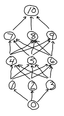
Your task: Compute $\dfrac{\partial E}{\partial w_{35}},$ $\dfrac{\partial E}{\partial w_{45}},$ $\dfrac{\partial E}{\partial w_{13}},$ $\dfrac{\partial E}{\partial w_{23}},$ $\dfrac{\partial E}{\partial w_{14}},$ $\dfrac{\partial E}{\partial w_{24}},$ $\dfrac{\partial E}{\partial w_{01}},$ and $\dfrac{\partial E}{\partial w_{02}}$ for the following network. (It's easiest to do it in that order.) Put your work in an Overleaf doc.
$$ \begin{matrix} & n_5 \\ & \nearrow \hspace{1.25cm} \nwarrow \\ n_3 & & n_4 \\ \uparrow & \nwarrow \hspace{1cm} \nearrow & \uparrow \\[-10pt] | & \diagdown \diagup & | \\[-10pt] | & \diagup \diagdown & | \\[-10pt] | & \diagup \hspace{1cm} \diagdown & | \\ n_1 & & n_2\\ & \nwarrow \hspace{1.25cm} \nearrow \\ & n_0 \\ \end{matrix} $$Show ALL your work! (If some work is the same as what you've already wrote down for a previous gradient computation, you can just put dot-dot-dot. But if you get stuck, then go back and write down all intermediate steps.) Also, make sure to use the simplest notation possible (for example, instead of writing $f_k(i_k),$ write $a_k$)
Check your answer by substituting the following values:
$$ y_\textrm{actual}=1 \qquad \begin{matrix} a_0 = 2 \\ a_1 = 3 \\ a_2 = 4 \\ a_3 = 5 \\ a_4 = 6 \\ a_5 = 7 \end{matrix} \qquad \begin{matrix} f_0'(i_0) = 8 \\ f_1'(i_1) = 9 \\ f_2'(i_2) = 10 \\ f_3'(i_3) = 11 \\ f_4'(i_4) = 12 \\ f_5'(i_5)=13 \end{matrix} \qquad \begin{matrix} w_{01} = 14 \\ w_{02} = 15 \\ w_{13} = 16 \\ w_{14} = 17 \\ w_{23} = 18 \\ w_{24} = 19 \\ w_{34} = 20 \\ w_{35} = 21 \\ w_{45} = 22 \end{matrix} $$You should get the following:
$$\begin{align*} \dfrac{\partial E}{\partial w_{35}} &= 780 \\[5pt] \dfrac{\partial E}{\partial w_{45}} &= 936 \\[5pt] \dfrac{\partial E}{\partial w_{13}} &= 108108 \\[5pt] \dfrac{\partial E}{\partial w_{23}} &= 144144 \\[5pt] \dfrac{\partial E}{\partial w_{14}} &= 123552 \\[5pt] \dfrac{\partial E}{\partial w_{24}} &= 164736 \\[5pt] \dfrac{\partial E}{\partial w_{01}} &= 22980672 \\[5pt] \dfrac{\partial E}{\partial w_{02}} &= 28622880 \end{align*}$$Future Problem
Compute $\dfrac{\textrm dE}{\textrm dw_{34}},$ $\dfrac{\textrm dE}{\textrm dw_{24}},$ $\dfrac{\textrm dE}{\textrm dw_{13}},$ $\dfrac{\textrm dE}{\textrm dw_{12}},$ and $\dfrac{\textrm dE}{\textrm dw_{01}}$ for the following network. (It's easiest to do it in that order.) Put your work in an Overleaf doc.
$$ \begin{matrix} & & n_4 \\ & \nearrow & & \nwarrow \\ n_2 & & & & n_3 \\ & \nwarrow & & \nearrow \\ & & n_1 \\ & & \uparrow \\ & & n_0 \\ \end{matrix} $$Show ALL your work! Also, make sure to use the simplest notation possible (for example, instead of writing $f_k(i_k),$ write $a_k$)
Check your answer by substituting the following values:
$$ y_\textrm{actual}=1 \qquad \begin{matrix} a_0 = 2 \\ a_1 = 3 \\ a_2 = 4 \\ a_3 = 5 \\ a_4 = 6 \end{matrix} \qquad \begin{matrix} f_0'(i_0) = 7 \\ f_1'(i_1) = 8 \\ f_2'(i_2) = 9 \\ f_3'(i_3) = 10 \\ f_4'(i_4) = 11 \end{matrix} \qquad \begin{matrix} w_{01} = 12 \\ w_{12} = 13 \\ w_{13} = 14 \\ w_{24} = 15 \\ w_{34} = 16 \end{matrix} $$You should get $$ \dfrac{\textrm dE}{\textrm d w_{34}} = 550, \qquad \dfrac{\textrm dE}{\textrm d w_{24}} = 440, \qquad \dfrac{\textrm dE}{\textrm d w_{13}} = 52800, \qquad \dfrac{\textrm dE}{\textrm d w_{12}} = 44550, \qquad \dfrac{\textrm dE}{\textrm d w_{01}} = 7031200. $$
Future Problem
Neural Net-Based Logistic Regressor
Make sure you get this problem done completely. Neural nets have a very steep learning curve and they're going to be sticking with us until the end of the semester.
a. Given $\sigma(x) = \dfrac{1}{1+e^{-x}},$ prove that $\sigma'(x) = \sigma(x) (1-\sigma(x)).$ Write this proof in an Overleaf doc.
b. In neural networks, neurons are often given "activation functions", where
node.activity = node.activation_function(weighted sum of inputs to node)In this problem, you'll extend your neural net to include activation functions. Then, you'll equip the neurons with activations so as to implement a logistic regressor.
>>> weights = {(0,2): -0.1, (1,2): 0.5}

>>> def linear_function(x):
        return x
>>> def linear_derivative(x):
        return 1
>>> def sigmoidal_function(x):
        return 1/(1+math.exp(-x))
>>> def sigmoidal_derivative(x):
        s = sigmoidal_function(x)
        return s * (1 - s)

>>> activation_types = ['linear', 'linear', 'sigmoidal']
>>> activation_functions = {
    'linear': {
        'function': linear_function,
        'derivative': linear_derivative
    },
    'sigmoidal': {
        'function': sigmoidal_function,
        'derivative': sigmoidal_derivative
    }
}

>>> nn = NeuralNetwork(weights, activation_types, activation_functions)

>>> data_points = [
    {'input': [1,0], 'output': [0.1]},
    {'input': [1,1], 'output': [0.2]},
    {'input': [1,2], 'output': [0.4]},
    {'input': [1,3], 'output': [0.7]}
    ]
>>> for i in range(1,10001):
        err = 0
        for data_point in data_points:
            nn.update_weights(data_point)
            err += nn.calc_squared_error(data_point)
        if i < 5 or i % 1000 == 0:
            print('iteration {}'.format(i))
            print('    gradient: {}'.format(nn.calc_gradient(data_point))
            print('    updated weights: {}'.format(nn.weights))
            print('    error: {}'.format(err))
            print()

iteration 1
    gradient: {(0, 2): 0.03184692266577955, (1, 2): 0.09554076799733865}
    updated weights: {(0, 2): -0.10537885784041535, (1, 2): 0.4945789883636697}
    error: 0.40480006957774683

iteration 2
    gradient: {(0, 2): 0.031126202300065627, (1, 2): 0.09337860690019688}
    updated weights: {(0, 2): -0.11072951375555531, (1, 2): 0.48919868238711295}
    error: 0.3989945995186133

iteration 3
    gradient: {(0, 2): 0.030367826123201307, (1, 2): 0.09110347836960392}
    updated weights: {(0, 2): -0.11605116651884796, (1, 2): 0.4838609744178689}
    error: 0.3932640005281893

iteration 4
    gradient: {(0, 2): 0.029572207383720784, (1, 2): 0.08871662215116236}
    updated weights: {(0, 2): -0.12134303561025003, (1, 2): 0.4785677220228999}
    error: 0.3876106111541695

iteration 1000
    gradient: {(0, 2): -0.04248103992359947, (1, 2): -0.12744311977079842}
    updated weights: {(0, 2): -1.441870816044744, (1, 2): 0.6320712307086241}
    error: 0.03103391055967604

iteration 2000
    gradient: {(0, 2): -0.026576913835657988, (1, 2): -0.07973074150697396}
    updated weights: {(0, 2): -1.8462575194764488, (1, 2): 0.8112377281576201}
    error: 0.010469324799663702

iteration 3000
    gradient: {(0, 2): -0.019389915442213898, (1, 2): -0.058169746326641694}
    updated weights: {(0, 2): -2.0580006793189596, (1, 2): 0.903267622168482}
    error: 0.004993174823452696

iteration 4000
    gradient: {(0, 2): -0.01536481706566838, (1, 2): -0.04609445119700514}
    updated weights: {(0, 2): -2.187017035077964, (1, 2): 0.9588032475551099}
    error: 0.002982405174006053

iteration 5000
    gradient: {(0, 2): -0.012858896793162088, (1, 2): -0.038576690379486266}
    updated weights: {(0, 2): -2.2717393677429842, (1, 2): 0.995065996436664}
    error: 0.00211991513136444

iteration 6000
    gradient: {(0, 2): -0.011201146193726709, (1, 2): -0.033603438581180124}
    updated weights: {(0, 2): -2.3298248394321606, (1, 2): 1.0198377357361068}
    error: 0.0017156674543843792

iteration 7000
    gradient: {(0, 2): -0.010062009597155228, (1, 2): -0.030186028791465685}
    updated weights: {(0, 2): -2.370740520022862, (1, 2): 1.037244660012689}
    error: 0.0015153961429219282

iteration 8000
    gradient: {(0, 2): -0.009259319779522148, (1, 2): -0.027777959338566444}
    updated weights: {(0, 2): -2.400083365137227, (1, 2): 1.0497070597284772}
    error: 0.0014124679719747604

iteration 9000
    gradient: {(0, 2): -0.008683873946383038, (1, 2): -0.026051621839149115}
    updated weights: {(0, 2): -2.4213875864199608, (1, 2): 1.058744505427183}
    error: 0.0013582149901490035

iteration 10000
    gradient: {(0, 2): -0.00826631063707707, (1, 2): -0.024798931911231212}
    updated weights: {(0, 2): -2.4369901278483534, (1, 2): 1.065357551487286}
    error: 0.001329102258719855

>>> nn.weights
should be close to
    {(0,2): -2.44, (1,2): 1.07}

because the data points all lie approximately on the sigmoid
    output = 1/(1 + e^(-(input[0] * -2.44 + input[1] * 1.07)) )
Super Important: You'll have to update your gradient descent to account for the activation functions. This will require using the chain rule. In our case, we'll have
squared_error = (y_predicted - y_actual)^2

d(squared_error)/d(weights)
    = 2 (y_predicted - y_actual) d(y_predicted - y_actual)/d(weights)
    = 2 (y_predicted - y_actual) [ d(y_predicted)/d(weights) - 0]
    = 2 (y_predicted - y_actual) d(y_predicted)/d(weights)

y_predicted
    = nodes[2].activity
    = nodes[2].activation_function(nodes[2].input)
    = nodes[2].activation_function(
        weights[(0,2)] * nodes[0].activity
        + weights[(1,2)] * nodes[1].activity
    )
    = nodes[2].activation_function(
        weights[(0,2)] * nodes[0].activation_function(nodes[0].input)
        + weights[(1,2)] * nodes[1].activation_function(nodes[1].input)
    )

d(y_predicted)/d(weights[(0,2)])
    = nodes[2].activation_derivative(nodes[2].input)
       * d(nodes[2].input)/d(weights[(0,2)])
    = nodes[2].activation_derivative(nodes[2].input)
      * d(weights[(0,2)] * nodes[0].activity + weights[(1,2)] * nodes[1].activity)/d(weights[(0,2)])
    = nodes[2].activation_derivative(nodes[2].input)
       * nodes[0].activity

by the same reasoning as above:

d(y_predicted)/d(weights[(1,2)]
    = nodes[2].activation_derivative(nodes[2].input)
       * nodes[1].activity
Note: If no activation_functions variable is passed in, then assume all activation functions are linear.
Future Problem
b. Time for an introduction to neural nets! In this problem, we'll create a really simple neural network that is essentially a "neural net"-style implementation of linear regression. We'll start off with something simple and familiar, but we'll implement much more advanced models in the near future.
Note: It seems like we need to merge our graph library into our machine-learning library. So, let's do that. The src your machine-learning library should now look like this:
src/
- models/
  - linear_regressor.py
  - neural_network.py
  - ...
- graphs/
  - weighted_graph.py
  - ...
(If you have a better idea for the structure of our library, feel free to do it your way and bring it up for discussion during the next class)
Create a NeuralNetwork class that inherits from weighted graph. Pass in dictionary of weights to determine connectivity and initial weights.
>>> weights = {(0,2): -0.1, (1,2): 0.5}
>>> nn = NeuralNetwork(weights)

This is a graphical representation of the model:

               nodes[2]                   ("output layer")
            ^            ^
           /              \
  weights[(0,2)]    weights[(1,2)]
        ^                    ^
       /                      \
nodes[0]                      nodes[1]     ("input layer")
To make a prediction, our simple neural net computes a weighted sum of the input values. (Again, this will become more involved in the future, but let's not worry about that just yet.)
>>> nn.predict([1,3])
1.4

    behind the scenes:

    assign nodes[0] a value of 1 and nodes[1] a value of 3,
    and then return the following:

    weights[(0,2)] * nodes[0].value + weights[(1,2)] * nodes[1].value
    = -0.1 * 1 + 0.5 * 3
    = 1.4
If we know the output that's supposed to be associated with a given input, we can compute the error in the prediction.
We'll use the squared error, so that we can frame the problem of fitting the neural network as "choosing weights which minimize the squared error".
To find the weights which minimize the squared error, we can perform gradient descent. As we'll see in the future, calculating the gradient of the weights can get a little tricky (it requires a technique called "backpropagation"). But for now, you can just hard-code the process for this particular network.
>>> data_point = {'input': [1,3], 'output': [7]}
>>> nn.calc_squared_error(data_point)
31.36     [ because (7-1.4)^2 = 5.6^2 = 31.36 ]

>>> nn.calc_gradient(data_point)
{(0,2): -11.2, (1,2): -33.6}

    behind the scenes:

    squared_error = (y_actual - y_predicted)^2

    d(squared_error)/d(weights)
        = 2 (y_actual - y_predicted) d(y_actual - y_predicted)/d(weights)
        = 2 (y_actual - y_predicted) [ 0 - d(y_predicted)/d(weights) ]
        = -2 (y_actual - y_predicted) d(y_predicted)/d(weights)

    remember that
        y_predicted = weights[(0,2)] * nodes[0].value + weights[(1,2)] * nodes[1].value

    so
        d(y_predicted)/d(weights[(0,2)]) = nodes[0].value
        d(y_predicted)/d(weights[(1,2)]) = nodes[1].value

    Therefore

        d(squared_error)/d(weights[(0,2)])
            = -2 (y_actual - y_predicted) d(y_predicted)/d(weights[(0,2)])
            = -2 (y_actual - y_predicted) nodes[0].value
            = -2 (7 - 1.4) (1)
            = -11.2

        d(squared_error)/d(weights[(1,2)])
            = -2 (y_actual - y_predicted) d(y_predicted)/d(weights[(1,2)])
            = -2 (y_actual - y_predicted) nodes[1].value
            = -2 (7 - 1.4) (3)
            = -33.6
Once we've got the gradient, we can update the weights using gradient descent.
>>> nn.update_weights(data_point, learning_rate=0.01)

    new_weights = old_weights - learning_rate * gradient
                = {(0,2): -0.1, (1,2): 0.5}
                   - 0.01 * {(0,2): -11.2, (1,2): -33.6}
                = {(0,2): -0.1, (1,2): 0.5}
                   + {(0,2): 0.112, (1,2): 0.336}
                = {(0,2): 0.012, (1,2): 0.836}
If we repeatedly loop through a dataset and update the weights for each data point, then we should get a model whose error is minimized.
Caveat: the minimum will be a local minimum, which is not guaranteed to be a global minimum.
Here is a test case with some data points that are on the line $y=1+2x.$ Our network is set up to fit any line of the form $y = \beta_0 \cdot 1 + \beta_1 \cdot x,$ where $\beta_0 = $ weights[(0,2)] and $\beta_1=$ weights[(1,2)].
Note that this line can be written as
output = 1 * input[0] + 2 * input[1]In this particular case, the weights should converge to the true values (1 and 2).
>>> weights = {(0,2): -0.1, (1,2): 0.5}
>>> nn = NeuralNetwork(weights)
>>> data_points = [
    {'input': [1,0], 'output': [1]},
    {'input': [1,1], 'output': [3]},
    {'input': [1,2], 'output': [5]},
    {'input': [1,3], 'output': [7]}
    ]
>>> for _ in range(1000):
        for data_point in data_points:
            nn.update_weights(data_point)

>>> nn.weights
should be really close to
    {(0,2): 1, (1,2): 2}

because the data points all lie on the line
    output = input[0] * 1 + input[1] * 2
Once you've got your final weights, post them on #results.
Future Problem
Primary problems; 60% of assignment grade; 90 minutes estimate
a. Assert that your decision trees pass some tests. (They likely will, so this problem will likely only take 10 minutes or so, I just to make sure we're all clear before we go back to improving our random forest, modeling real-world datasets, and moving on to neural nets.)
(i) Assert that BOTH your gini decision tree and random decision tree pass the following test.
Create a dataset consisting of 100 points $$ \Big[ (x,y,\textrm{label}) \mid x,y \in \mathbb{Z}, \,\, -5 \leq x,y \leq 5, \,\, xy \neq 0 \big], $$ where $$ \textrm{label} = \begin{cases} \textrm{positive}, \quad x>0, y > 0 \\ \textrm{negative}, \quad \textrm{otherwise} \end{cases} $$
Predict the label of this dataset. Train on 100% of the data and test on 100% of the data.
You should get an accuracy of 100%.
You should have exactly 2 splits
Note: Your tree should look exactly like one of these:
           split y=0
         /          \
     y < 0         y > 0
    pure neg      split x=0
                    /   \
                x < 0   x > 0
              pure neg  pure pos
.
or
.
           split x=0
         /          \
     x < 0         x > 0
    pure neg      split y=0
                    /   \
                y < 0   y > 0
              pure neg  pure pos
(ii) Assert that your gini decision tree passes Tests 1,2,3,4 from problem 84-1.
(iii) Assert that your random forest with 10 trees passes Tests 1,2,3,4 from problem 84-1.
Future Problem
b. Assert that your random decision tree passes the following tests.
Test 1
Create a dataset consisting of 100 points $$ \Big[ (x,y,\textrm{label}) \mid x,y \in \mathbb{Z}, \,\, -5 \leq x,y \leq 5, \,\, xy \neq 0 \big], $$ where $$ \textrm{label} = \begin{cases} \textrm{positive}, \quad xy > 0 \\ \textrm{negative}, \quad xy < 0 \end{cases} $$
Train a random decision tree to predict the label of this dataset. Train on 100% of the data and test on 100% of the data. You should get an accuracy of 100%.
Test 2
Create a dataset consisting of 150 points $$ \begin{align*} &\Big[ (x,y,\textrm{A}) \mid x,y \in \mathbb{Z}, \,\, -5 \leq x,y \leq 5, \,\, xy \neq 0 \Big] \\ &+ \Big[ (x,y,\textrm{B}) \mid x,y \in \mathbb{Z}, \,\, 1 \leq x,y \leq 5 \Big] \\ &+ \Big[ (x,y,\textrm{B}) \mid x,y \in \mathbb{Z}, \,\, 1 \leq x,y \leq 5 \Big]. \end{align*} $$ This dataset consists of $100$ data points labeled "A" distributed evenly throughout the plane and $50$ data points labeled "B" in quadrant I. Each integer pair in quadrant I will have $1$ data point labeled "A" and $2$ data points labeled "B".
Train a random decision tree to predict the label of this dataset. Train on 100% of the data and test on 100% of the data. You should get an accuracy of 83.3% (25/150 misclassified)
Test 3
Create a dataset consisting of 1000 points $$ \Big[ (x,y,z,\textrm{label}) \mid x,y,z \in \mathbb{Z}, \,\, -5 \leq x,y,z \leq 5, \,\, xyz \neq 0 \big], $$ where $$ \textrm{label} = \begin{cases} \textrm{positive}, \quad xyz > 0 \\ \textrm{negative}, \quad xyz < 0 \end{cases} $$
Train a random decision tree to predict the label of this dataset. Train on 100% of the data and test on 100% of the data. You should get an accuracy of 100%.
Note: These are a lot of data points, but the tree won't need to do many splits, so the code should run quickly. If the code takes a long time to run, it means you've got an issue, and you should post on Slack if you can't figure out why it's taking so long.
Test 4
Create a dataset consisting of 1250 points $$ \begin{align*} &\Big[ (x,y,z,\textrm{A}) \mid x,y,z \in \mathbb{Z}, \,\, -5 \leq x,y,z \leq 5, \,\, xyz \neq 0 \Big] \\ &+ \Big[ (x,y,z,\textrm{B}) \mid x,y,z \in \mathbb{Z}, \,\, 1 \leq x,y,z \leq 5 \Big] \\ &+ \Big[ (x,y,z,\textrm{B}) \mid x,y,z \in \mathbb{Z}, \,\, 1 \leq x,y,z \leq 5 \Big]. \end{align*} $$ This dataset consists of $1000$ data points labeled "A" distributed evenly throughout the eight octants and $250$ data points labeled "B" in octant I. Each integer pair in octant I will have $1$ data point labeled "A" and $2$ data points labeled "B".
Train a random decision tree to predict the label of this dataset. Train on 100% of the data and test on 100% of the data. You should get an accuracy of 90% (125/1250 misclassified)
Note: These are a lot of data points, but the tree won't need to do many splits, so the code should run quickly. If the code takes a long time to run, it means you've got an issue, and you should post on Slack if you can't figure out why it's taking so long.
Future Problem
Primary problems; 45% of assignment grade; 75 minutes estimate
a. You'll need to do part 1 of the supplemental problem before you do this problem.
(i) Download the freshman_lbs.csv dataset from https://people.sc.fsu.edu/~jburkardt/data/csv/csv.html, read it into a DataFrame, and create 5 test-train splits:
- Testing data = first 20% of the records, training data = remaining 80%
- Testing data = second 20% of the records, training data = remaining 80%
- Testing data = third 20% of the records, training data = remaining 80%
- Testing data = fourth 20% of the records, training data = remaining 80%
- Testing data = fifth 20% of the records, training data = remaining 80%
Note that you'll need to convert the appropriate entries to numbers (instead of strings) in the dataset. There are 2 options for doing this:
Option 1: don't worry about fixing the format within the
read_csvmethod. Just do something likedf = df.apply('weight', lambda x: int(x))afterwards, before you pass the dataframe into your model.Option 2: when you read in the csv, after you do the
lines = file.read().split('\n')
entries = [line.split(',') for line in lines]
thing, you can loop through the entries, and if
entry[0]+entry[-1] == '""', then you can setentry = entry[1:-1]to remove the quotes. Otherwise, ifentry[0]+entry[-1] != '""', then you can try to doentry = float(entry[1:-1]).
(ii) For each test-train split, fit each of the following models on the training data and use it to predict the sexes on the testing data. (You are predicting sex as a function of weight and BMI, and you can just use columns corresponding to September data.)
Decision tree using Gini split criterion
A single random decision tree
Random forest with 10 trees
Random forest with 100 trees
Random forest with 1000 trees
(iii) For each model, compute the accuracy (count the total number of correct classifications and divide by the total number of classifications). Put these results in a table in an Overleaf document.
Note that the total number of classifications should be equal to the total number of records in the dataset (you did 5 train-test splits, and each train-test split involved testing on 20% of the data).
(iv) Below the table, analyze the results. Did you expect these results, or did they surprise you? Why do you think you got the results you did?
b. For each of your classmates, copy over their DumbStrategy and CombatStrategy and run your DumbPlayer/CombatPlayer tests using your classmate's strategy. Fill out the following information for each classmate:
Name of classmate
When you copied over their
DumbStrategyand ran your DumbPlayer tests, did they pass? If not, then what's the issue? Is it a problem with your game, or with their strategy class?When you copied over their
CombatStrategyand ran your CombatPlayer tests, did they pass? If not, then what's the issue? Is it a problem with your game, or with their strategy class?
Future Problem
Location: machine-learning/src/decision_tree.py
Grade Weighting: 40%
Update your DecisionTree to have the option to build the tree via random splits. By "random splits", I mean that the tree should randomly choose from the possible splits, and it should keep splitting until each leaf node is pure.
>>> dt = DecisionTree(split_metric = 'gini')
>>> dt.fit(df)
Fits the decision tree using the Gini metric

>>> dt = DecisionTree(split_metric = 'random')
>>> dt.fit(df)
Fits the decision tree by randomly choosing splits
Future Problem
Estimated Time: 15 minutes
Location:
machine-learning/analysis/scatter_plot.py
Points: 5
Make a scatter plot of the following dataset consisting of the points (x, y, class). When the class is A, color the dot red. When it is B, color the dot blue. Post your plot on slack once you've got it.
data = [[2,13,'B'],[2,13,'B'],[2,13,'B'],[2,13,'B'],[2,13,'B'],[2,13,'B'],
    [3,13,'B'],[3,13,'B'],[3,13,'B'],[3,13,'B'],[3,13,'B'],[3,13,'B'],
    [2,12,'B'],[2,12,'B'],
    [3,12,'A'],[3,12,'A'],
    [3,11,'A'],[3,11,'A'],
    [3,11.5,'A'],[3,11.5,'A'],
    [4,11,'A'],[4,11,'A'],
    [4,11.5,'A'],[4,11.5,'A'],
    [2,10.5,'A'],[2,10.5,'A'],
    [3,10.5,'B'],
    [4,10.5,'A']]
In the plot, make the dot size proportional to the number of points at that location.
For example, to plot a data set
[
 (1,1),
 (2,4), (2,4),
 (3,9), (3,9), (3,9), (3,9),
 (4,16), (4,16), (4,16), (4,16), (4,16), (4,16), (4,16), (4,16), (4,16)
 ]
you would use the following code:
import matplotlib.pyplot as plt
plt.scatter(x=[1, 2, 3, 4], y=[1, 4, 9, 16], s=[20, 40, 80, 160], c='red')

Future Problem
Estimated Time: 10-60 minutes (depending on whether you've got bugs)
Location:
machine-learning/src/decision_tree.py
machine-learning/tests/test_decision_tree.py
Points: 10
Refactor your DecisionTree so that the dataframe is passed in the fit method (not when the decision tree is initialized). Also, create a method to classify points.
Then, make sure decision tree passes the following tests, using the data from problem 71-1.
Note: Based on visually inspecting a plot of the data, I think these tests are correct, but if you get something different (that looks reasonable), post on Slack so I can check.
df = DataFrame.from_array(data, columns = ['x', 'y', 'class'])

>>> dt = DecisionTree()
>>> dt.fit(df)

The tree should look like this:

                           (13A, 15B)
                            /      \
                  (y < 12.5)       (y >= 12.5)
                  (13A, 3B)        (12B)
                  /         \
          (x < 2.5)          (x >= 2.5)
          (2A, 2B)                (11A, 1B)
         /     \                  /        \
(y < 11.25)   (y >= 11.25)  (y < 10.75)     (y >= 10.75)
(2A)          (2B)          (1A, 1B)        (10A)
                            /      \
                   (x < 3.5)        (x >= 3.5)
                        (1B)        (1A)

>>> dt.root.best_split
('y', 12.5)
>>> dt.root.low.best_split
('x', 2.5)
>>> dt.root.low.low.best_split
('y', 11.25)
>>> dt.root.low.high.best_split
('y', 10.75)
>>> dt.root.low.high.low.best_split
('x', 3.5)

>>> dt.classify({'x': 2, 'y': 11.5})
'B'
>>> dt.classify({'x': 2.5, 'y': 13})
'B'
>>> dt.classify({'x': 4, 'y': 12})
'A'
>>> dt.classify({'x': 3.25, 'y': 10.5})
'B'
>>> dt.classify({'x': 3.75, 'y': 10.5})
'A'
Future Problem
Estimated Time: 45 minutes
Location:
machine-learning/src/decision_tree.py
machine-learning/tests/test_decision_tree.py
Points: 15
If you haven't already, create a split() method in your DecisionTree (not the same as the split() method in your Node!) that splits the tree at the node with highest impurity.
Then, create a fit() method in your DecisionTree that keeps on split()-ing until all terminal nodes are completely pure.
Assert that the following tests pass:
>>> df = DataFrame.from_array(
    [[1, 11, 'A'],
    [1, 12, 'A'],
    [2, 11, 'A'],
    [1, 13, 'B'],
    [2, 13, 'B'],
    [3, 13, 'B'],
    [3, 11, 'B']],
    columns = ['x', 'y', 'class']
)
>>> dt = DecisionTree(df)

# currently, the decision tree looks like this:

                      (3A, 4B)

>>> dt.split()
# now, the decision tree looks like this:

                      (3A, 4B)
                      /      \
            (y < 12.5)       (y >= 12.5)
            (3A, 1B)         (3B)

>>> dt.split()
# now, the decision tree looks like this:

                    (3A, 4B)
                    /      \
           (y < 12.5)       (y >= 12.5)
           (3A, 1B)         (3B)
         /         \
(x < 2.5)          (x >= 2.5)
(3A)               (1B)

>>> dt.root.high.row_indices
[3, 4, 5]
>>> dt.root.low.low.row_indices
[0, 1, 2]
>>> dt.root.low.high.row_indices
[6]

>>> dt = DecisionTree(df)

# currently, the decision tree looks like this:

                      (3A, 4B)

>>> dt.fit()
# now, the decision tree looks like this:

                    (3A, 4B)
                    /      \
           (y < 12.5)       (y >= 12.5)
           (3A, 1B)         (3B)
         /         \
(x < 2.5)          (x >= 2.5)
(3A)               (1B)

>>> dt.root.high.row_indices
[3, 4, 5]
>>> dt.root.low.low.row_indices
[0, 1, 2]
>>> dt.root.low.high.row_indices
[6]
Future Problem
Estimated time: 60 min
Grading: 10 points
Locations:
machine-learning/src/leave_one_out_cross_validator.py
machine-learning/tests/test_leave_one_out_cross_validator.py
Write a class LeaveOneOutCrossValidator that computes percent_accuracy (also known as "leave-one-out cross validation") for any input classifier. For a refresher, see problem 58-1.
Assert that LeaveOneOutCrossValidator passes the following tests:
>>> df = the cookie dataset that's in test_k_nearest_neighbors_classifier.py
>>> knn = KNearestNeighborsClassifier(k=5)

>>> cv = LeaveOneOutCrossValidator(knn, df, prediction_column='Cookie Type')
    [ Note: under the hood, the LeaveOneOutCrossValidator should
      create a leave_one_out_df and do
      knn.fit(leave_one_out_df, prediction_column='Cookie Type') ]

>>> cv.accuracy()
0.7894736842105263 (Updated!)

Note: the following is included to help you debug.
Row 0 -- True Class is Shortbread; Predicted Class was Shortbread
Row 1 -- True Class is Shortbread; Predicted Class was Shortbread
Row 2 -- True Class is Shortbread; Predicted Class was Shortbread
Row 3 -- True Class is Shortbread; Predicted Class was Shortbread
Row 4 -- True Class is Sugar; Predicted Class was Sugar
Row 5 -- True Class is Sugar; Predicted Class was Sugar
Row 6 -- True Class is Sugar; Predicted Class was Sugar
Row 7 -- True Class is Sugar; Predicted Class was Shortbread
Row 8 -- True Class is Sugar; Predicted Class was Shortbread
Row 9 -- True Class is Sugar; Predicted Class was Sugar
Row 10 -- True Class is Fortune; Predicted Class was Fortune (Updated!)
Row 11 -- True Class is Fortune; Predicted Class was Fortune
Row 12 -- True Class is Fortune; Predicted Class was Fortune
Row 13 -- True Class is Fortune; Predicted Class was Shortbread
Row 14 -- True Class is Fortune; Predicted Class was Fortune (Updated!)
Row 15 -- True Class is Shortbread; Predicted Class was Sugar
Row 16 -- True Class is Shortbread; Predicted Class was Shortbread
Row 17 -- True Class is Shortbread; Predicted Class was Shortbread
Row 18 -- True Class is Shortbread; Predicted Class was Shortbread

>>> accuracies = []
>>> for k in range(1, len(data)-1):
>>>    knn = KNearestNeighborsClassifier(k)
>>>    cv = LeaveOneOutCrossValidator(knn, df, prediction_column='Cookie Type')
>>>    accuracies.append(cv.accuracy())

>>> accuracies
 [0.5789473684210527,
 0.5789473684210527, #(Updated!)
 0.5789473684210527,
 0.5789473684210527,
 0.7894736842105263, #(Updated!)
 0.6842105263157895,
 0.5789473684210527,
 0.5789473684210527, #(Updated!)
 0.6842105263157895, #(Updated!)
 0.5263157894736842,
 0.47368421052631576, #(Updated!)
 0.42105263157894735,
 0.42105263157894735, #(Updated!)
 0.3684210526315789, #(Updated!)
 0.3684210526315789, #(Updated!)
 0.3684210526315789, #(Updated!)
 0.42105263157894735]
Future Problem
Estimated Time: 2-3 hours
Location:
machine-learning/src/decision_tree.py
machine-learning/tests/test_decision_tree.py
Points: 15
In this problem, you will create the first iteration of a class DecisionTree that builds a decision tree by repeatedly looping through all possible splits and choosing the split with the highest "goodness of split".
We will use the following simple dataset:
['x', 'y', 'class']
[1, 11, 'A']
[1, 12, 'A']
[2, 11, 'A']
[1, 13, 'B']
[2, 13, 'B']
[3, 12, 'B']
[3, 13, 'B']
For this dataset, "all possible splits" mean all midpoints between distinct entries in sorted data columns.
The sorted distinct entries of
xare 1, 2, 3.The sorted distinct entries of
yare 11, 12, 13.
So, "all possible splits" are x=1.5, x=2.5, y=11.5, y=12.5.
Assert that the following tests pass. Note that you will need to create a Node class for the nodes in your decision tree.
>>> df = DataFrame.from_array(
    [[1, 11, 'A'],
    [1, 12, 'A'],
    [2, 11, 'A'],
    [1, 13, 'B'],
    [2, 13, 'B'],
    [3, 13, 'B'],
    [3, 11, 'B']],
    columns = ['x', 'y', 'class']
)
>>> dt = DecisionTree(df)

>>> dt.root.row_indices
[0, 1, 2, 3, 4, 5, 6] # these are the indices of data points in the root node

>>> dt.root.class_counts
{
    'A': 3,
    'B': 4
}

>>> dt.root.impurity
0.490 # rounded to 3 decimal places

>>> dt.root.possible_splits.to_array()
# dt.possible_splits is a dataframe with columns
# ['feature', 'value', 'goodness of split']
# Note: below is rounded to 3 decimal places

[['x', 1.5,  0.085],
 ['x', 2.5,  0.147],
 ['y', 11.5, 0.085],
 ['y', 12.5, 0.276]]

>>> dt.root.best_split
('y', 12.5)

>>> dt.root.split()
# now, the decision tree looks like this:

                      (3A, 4B)
                      /      \
            (y < 12.5)       (y >= 12.5)
            (3A, 1B)         (3B)

# "low" refers to the "<" child node
# "high" refers to the ">=" child node
>>> dt.root.low.row_indices
[0, 1, 2, 6]
>>> dt.root.high.row_indices
[3, 4, 5]

>>> dt.root.low.impurity
0.375
>>> dt.root.high.impurity
0

>>> dt.root.low.possible_splits.to_array()

[['x', 1.5,  0.125],
 ['x', 2.5,  0.375],
 ['y', 11.5, 0.042]]

>>> dt.root.low.best_split
('x', 2.5)

>>> dt.root.low.split()
# now, the decision tree looks like this:

                    (3A, 4B)
                    /      \
           (y < 12.5)       (y >= 12.5)
           (3A, 1B)         (3B)
         /         \
(x < 2.5)          (x >= 2.5)
(3A)               (1B)

>>> dt.root.low.low.row_indices
[0, 1, 2]
>>> dt.root.low.high.row_indices
[6]

>>> dt.root.low.low.impurity
0
>>> dt.root.low.high.impurity
0
Future Problem
Estimated time: 60 min
Location: assignment-problems/quicksort.py
Grading: 10 points
Previously, you wrote a variant of quicksort that involved splitting the list into two parts (one part $\leq$ the pivot, and another part $>$ the pivot), and then recursively calling quicksort on those parts.
However, this algorithm can be made more efficient by keeping everything in the same list (rather than creating two new lists). You can do this by swapping elements rather than breaking them out into new lists.
Your task is to write a quicksort algorithm that uses only one list, and uses swaps to re-order elements within that list, per the quicksort algorithm. Here is an example of how to do that.
Make sure your algorithm passes the same test as the quicksort without swaps (that you did on the previous assignment).
Future Problem
Grading: 10 points
Create a class NaiveBayesClassifier withing machine-learning/src/naive_bayes_classifier.py that passes the following tests. These tests should be written in tests/test_naive_bayes_classifier.py using assert statements.
>>> df = DataFrame.from_array(
    [
        [False, False, False],
        [True, True, True],
        [True, True, True],
        [False, False, False],
        [False, True, False],
        [True, True, True],
        [True, False, False],
        [False, True, False],
        [True, False, True],
        [False, True, False]
    ]
    columns = ['errors', 'links', 'scam']
)
>>> naive_bayes = NaiveBayesClassifier(df, dependent_variable='scam')

>>> naive_bayes.probability('scam', True)
0.4
>>> naive_bayes.probability('scam', False)
0.6

>>> naive_bayes.conditional_probability(('errors',True), given=('scam',True))
1.0
>>> naive_bayes.conditional_probability(('links',False), given=('scam',True))
0.25

>>> naive_bayes.conditional_probability(('errors',True), given=('scam',False))
0.16666666666666666
>>> naive_bayes.conditional_probability(('links',False), given=('scam',False))
0.5

>>> observed_features = {
    'errors': True,
    'links': False
}
>>> naive_bayes.likelihood(('scam',True), observed_features)
0.1
>>> naive_bayes.likelihood(('scam',False), observed_features)
0.05

>>> naive_bayes.classify('scam', observed_features)
True

Note: in the event of a tie, choose the dependent variable that occurred most frequently in the dataset.
Future Problem
Grading: 10 points
Location: assignment-problems/quicksort_without_swaps.py
Implement a function quicksort that implements the variant of quicksort described here: https://www.youtube.com/watch?v=XE4VP_8Y0BU
- Note: this variant of
quicksortis very similar tomergesort.
Use your function to sort the list [5,8,-1,9,10,3.14,2,0,7,6] (write a test with an assert statement). Choose the pivot as the rightmost entry.
Future Problem
Location: Overleaf
Grading: 10 points
Construct a decision tree model for the following data. Include the Gini impurity and goodness of split at each node. You should choose the splits so as to maximize the goodness of split each time. Also, draw a picture of the decision boundary on the graph.
Future Problem
Location: Overleaf
Grading: 10 points
Construct a decision tree model for the following data, using the splits shown.
Remember that the formula for Gini impurity for a group with class distribution $\vec p$ is
$$ G(\vec p) = \sum_i p_i (1-p_i) $$and that the "goodness-of-split" is quantified as
$$ \text{goodness} = G(\vec p_\text{pre-split}) - \sum_\text{post-split groups} \dfrac{N_\text{group}}{N_\text{pre-split}} G(\vec p_\text{group}). $$See the updated Eurisko Assignment Template for an example of constructing a decision tree in latex for a graph with given splits.
Be sure to include the class counts, impurity, and goodness of split at each node
Be sure to label each edge with the corresponding decision criterion.
Future Problem
Neural Nets
Notation
$n_k$ - the $k$th neuron
$a_k$ - the activity of the $k$th neuron
$i_k$ - the input to the $k$th neuron. This is the weighted sum of activities of the parents of $n_k.$ If $n_k$ has no parents, then $i_k$ comes from the data directly.
$f_k$ - the activation function of the $k$th neuron. Note that in general, we have $a_k = f_k(i_k)$
$w_{k \ell}$ - the weight of the connection $n_k \to n_\ell.$ In your code, this is
weights[(k,l)].$E = (y_\textrm{predicted} - y_\textrm{actual})^2$ is the squared error that results from using the neural net to predict the value of the dependent variable, given values of the independent variables
$w_{k \ell} \to w_{k \ell} - \alpha \dfrac{\textrm dE}{\textrm dw_{k\ell}}$ is the gradient descent update, where $\alpha$ is the learning rate
Example
For a simple network $$ \begin{matrix} & & n_2 \\ & \nearrow & & \nwarrow \\ n_0 & & & & n_1,\end{matrix} $$ we have:
$$\begin{align*} y_\textrm{predicted} &= a_2 \\ &= f_2(i_2) \\ &= f_2(w_{02} a_0 + w_{12} a_1) \\ &= f_2(w_{02} f_0(i_0) + w_{12} f_1(i_1) ) \\ \\ \dfrac{\textrm dE}{\textrm dw_{02}} &= \dfrac{\textrm d}{\textrm dw_{02}} \left[ (y_\textrm{predicted} - y_\textrm{actual})^2 \right] \\ &= \dfrac{\textrm d}{\textrm dw_{02}} \left[ (a_2 - y_\textrm{actual})^2 \right] \\ &= 2(a_2 - y_\textrm{actual}) \dfrac{\textrm d}{\textrm dw_{02}} \left[ a_2 - y_\textrm{actual} \right] \\ &= 2(a_2 - y_\textrm{actual}) \dfrac{\textrm d }{\textrm dw_{02}} \left[ a_2 \right] \\ &= 2(a_2 - y_\textrm{actual}) \dfrac{\textrm d }{\textrm dw_{02}} \left[ f_2(i_2) \right] \\ &= 2(a_2 - y_\textrm{actual}) f_2'(i_2) \dfrac{\textrm d }{\textrm dw_{02}} \left[ i_2 \right] \\ &= 2(a_2 - y_\textrm{actual}) f_2'(i_2) \dfrac{\textrm d }{\textrm dw_{02}} \left[ w_{02} a_0 + w_{12} a_1 \right] \\ &= 2(a_2 - y_\textrm{actual}) f_2'(i_2) \dfrac{\textrm d }{\textrm dw_{02}} \left[ w_{02} a_0 + w_{12} a_1 \right] \\ &= 2(a_2 - y_\textrm{actual}) f_2'(i_2) a_0 \\ \\ \dfrac{\textrm dE}{\textrm dw_{12}} &= 2(a_2 - y_\textrm{actual}) f_2'(i_2) a_1 \end{align*}$$THE ACTUAL PROBLEM STATEMENT
Compute $\dfrac{\textrm dE}{\textrm dw_{23}},$ $\dfrac{\textrm dE}{\textrm dw_{12}},$ and $\dfrac{\textrm dE}{\textrm dw_{01}}$ for the following network. (It's easiest to do it in that order.) Put your work in an Overleaf doc.
$$ \begin{matrix} n_3 \\ \uparrow \\ n_2 \\ \uparrow \\ n_1 \\ \uparrow \\ n_0 \end{matrix} $$Show ALL your work! Also, make sure to use the simplest notation possible (for example, instead of writing $f_k(i_k),$ write $a_k$)
Check your answer by substituting the following values:
$$ y_\textrm{actual}=1 \qquad \begin{matrix} a_0 = 2 \\ a_1 = 3 \\ a_2 = 4 \\ a_3 = 5 \end{matrix} \qquad \begin{matrix} f_0'(i_0) = 6 \\ f_1'(i_1) = 7 \\ f_2'(i_2) = 8 \\ f_3'(i_3) = 9 \end{matrix} \qquad \begin{matrix} w_{01} = 10 \\ w_{12} = 11 \\ w_{23} = 12 \end{matrix} $$You should get $$ \dfrac{\textrm dE}{\textrm d w_{23}} = 288, \qquad \dfrac{\textrm dE}{\textrm d w_{12}} = 20736, \qquad \dfrac{\textrm dE}{\textrm d w_{01}} = 1064448. $$
Note: On the next couple assignments, we'll do the same exercise with progressively more advanced networks. This problem is relatively simple so that you have a chance to get used to working with the notation.
Space Empires
Finish creating your game level 3 strategy. (See problem 93-1 for a description of game level 3, which you should have implemented by now.) Then, implement the following strategy and run it against your level 3 strategy:
NumbersBerserkerLevel3- always buys as many scouts as possible, and each time it buys a scout, immediately sends it on a direct route to attack the opponent.
Post on #machine-learning with your strategy's stats against these strategies:
MyStrategy vs NumbersBerserker
- MyStrategy win rate: __%
- MyStrategy loss rate: __%
- draw rate: __%
On the next assignment, we'll have the official matchups.
Future Problem
Location: Overleaf
Grading: 12 points
Naive Bayes classification is a way to classify a new observation consisting of multiple features, if we have data about how other observations were classified. It involves choosing the class that maximizes the posterior distribution of the classes, given the observation.
$$\begin{align*} \text{class} &= \underset{\text{class}}{\arg\max} \, P(\text{class} \, | \, \text{observed features}) \\ &= \underset{\text{class}}{\arg\max} \, \dfrac{P(\text{observed features} \, | \, \text{class}) P(\text{class})}{P(\text{observed features})} \\ &= \underset{\text{class}}{\arg\max} \, P(\text{observed features} \, | \, \text{class}) P(\text{class})\\ &= \underset{\text{class}}{\arg\max} \, \prod\limits_{\text{observed}\\ \text{features}} P(\text{feature} \, | \, \text{class}) P(\text{class})\\ &= \underset{\text{class}}{\arg\max} \, P(\text{class}) \prod\limits_{\text{observed}\\ \text{features}} P(\text{feature} \, | \, \text{class}) \\ \end{align*}$$The key assumption (used in the final line) is that all the features are independent:
$$\begin{align*} P(\text{observed features} \, | \, \text{class}) = \prod\limits_{\text{observed} \\ \text{features}} P(\text{feature} \, | \, \text{class}) \end{align*}$$Suppose that you want to find a way to classify whether an email is a phishing scam or not, based on whether it has errors and whether it contains links.
After checking 10 emails in your inbox, you came up with the following data set:
- No errors, no links; NOT scam
- Contains errors, contains links; SCAM
- Contains errors, contains links; SCAM
- No errors, no links; NOT scam
- No errors, contains links; NOT scam
- Contains errors, contains links; SCAM
- Contains errors, no links; NOT scam
- No errors, contains links; NOT scam
- Contains errors, no links; SCAM
- No errors, contains links; NOT scam
Now, you look at 4 new emails. For each of the new emails, compute
$$ P(\text{scam}) \prod\limits_{\text{observed}\\ \text{features}} P(\text{feature} \, | \, \text{scam}) \\[10pt] \text{and} \\[10pt] P(\text{not scam}) \prod\limits_{\text{observed}\\ \text{features}} P(\text{feature} \, | \, \text{not scam}) $$and decide whether it is a scam.
a. No errors, no links. You should get
$$ P(\text{scam}) \prod\limits_{\text{observed}\\ \text{features}} P(\text{feature} \, | \, \text{scam}) = 0 \\[10pt] \text{and} \\[10pt] P(\text{not scam}) \prod\limits_{\text{observed}\\ \text{features}} P(\text{feature} \, | \, \text{not scam}) = \dfrac{1}{4}. $$b. Contains errors, contains links. You should get
$$ P(\text{scam}) \prod\limits_{\text{observed}\\ \text{features}} P(\text{feature} \, | \, \text{scam}) = \dfrac{3}{10} \\[10pt] \text{and} \\[10pt] P(\text{not scam}) \prod\limits_{\text{observed}\\ \text{features}} P(\text{feature} \, | \, \text{not scam}) = \dfrac{1}{20}. $$c. Contains errors, no links. You should get
$$ P(\text{scam}) \prod\limits_{\text{observed}\\ \text{features}} P(\text{feature} \, | \, \text{scam}) = \dfrac{1}{10} \\[10pt] \text{and} \\[10pt] P(\text{not scam}) \prod\limits_{\text{observed}\\ \text{features}} P(\text{feature} \, | \, \text{not scam}) = \dfrac{1}{20}. $$d. No errors, contains links. You should get
$$ P(\text{scam}) \prod\limits_{\text{observed}\\ \text{features}} P(\text{feature} \, | \, \text{scam}) = 0 \\[10pt] \text{and} \\[10pt] P(\text{not scam}) \prod\limits_{\text{observed}\\ \text{features}} P(\text{feature} \, | \, \text{not scam}) = \dfrac{1}{4}. $$Future Problem
Space empires
Future Problem
Build tic tac toe playing agent that uses game tree, always moving in direction of highest win probability.
should win the vast majority of the time versus random player
Future Problem
Build game tree for tic tac toe
https://www2.lv.psu.edu/ojj/courses/ist-230/students/math/2002-1-db-mc-lc/game_trees.htm
Future Problem
logistic regressor - normalizing variables
upcoming quiz - for titanic modeling, review what we did and make sure you understand why we did it
Future Problem
Logistic regressor - pruning
https://github.com/eurisko-us/problem-output-generation/blob/master/titanic/analysis.py
talk about checkpoints for when repl.it craps out
log for debugging purposes:
Minimax Algorithm
exercise by hand
KNN
Fit the titanic surival dataset using sklearn's k-nearest neighbors classifier.
table with train & test accuracies for k=5, 15, 25
Using all non-interaction features
Backwards selection on non-interaction features
Get the baseline training/testing accuracy using the non-interaction
use k=5, 15, 25
Future Problem
alpha-beta pruning
Problem 97
Before you start this problem, make a copy of your blog post tex file.
Take one last read through your blog post.
We've let it sit for a while, so you should see some areas for improvement coming back to it with fresh eyes.
At the end of this assignment you should be 100% done with your blog post. It should be finalized to the point that it's ready for other students/people to read.
Copy/paste your old tex file and updated tex file into https://www.diffchecker.com/ so that I can see what you updated. Then, submit a link to the log (just like you did for Space Empires logs).
The Final
The final will take place on Wednesday 6/2 from 11am-1pm. Any topic that appeared on an assignment this semester is fair game.
Here are the notes from class. (I'll update this with more notes as we do more review.)
Here is a list of topics to help you focus your studying.
- basics of haskell & C++
- numpy, pandas, sklearn
- all the models we've covered (in particular: linear/logistic regression, polynomial regression, k-nearest neighbors, k-means clustering)
- breadth-first and depth-first search
- roulette probability selection
- hill climbing (as a general concept)
- logistic regression when the target variable has 0's and/or 1's
- fitting logistic regression via gradient descent
- integral estimation (left, right, midpoint, trapezoidal, Simpson's)
- Euler estimation
- predator-prey and SIR modeling
- interaction terms, indicator (dummy) variables
- underfitting/overfitting
- distance/shortest paths in graphs
- dijkstra's algorithm
- train/test datasets
- using linear regression with nonlinear functions
- titanic analysis
- cross-validation
- normalization
- clustering
Problem 96
Create an elbow curve for k-means clustering on the titanic dataset, using min-max normalization.
Remember that the titanic dataset is provided here:
In your clustering, use all the rows of the data set, but only these columns:
["Sex", "Pclass", "Fare", "Age", "SibSp"]The first few rows of the normalized data set should be as follows:
["Sex", "Pclass", "Fare", "Age", "SibSp"]
[0, 1, 0.01415106, 0.27117366, 0.125]
[1, 0, 0.13913574, 0.4722292,  0.125]
[1, 1, 0.01546857, 0.32143755, 0]
Then, just as before, make a plot of sum squared distance to cluster centers vs $k$ for k=[1,2,3,...,25].
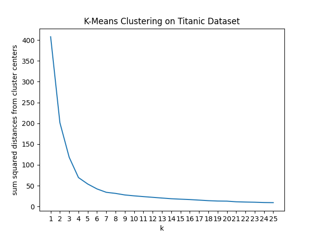
Choose k to be at the elbow of the graph (looks like k=4). Then, fit a k-means model with k=4, add the cluster label as a column in your data set, and find the column averages.
Tip: Use groupby: df.groupby(['cluster']).mean()
Here is an example of the format for your output. Your numbers might be different.
              Sex    Pclass       Fare        Age     SibSp
cluster
0        1.000000  2.183908  38.759867  28.815940  0.000000
1        0.502110  2.092827  45.046011  29.253985  1.118143
2        0.456522  2.847826  52.115039  14.601963  4.369565
3        0.000000  2.419355  20.452848  31.896441  0.000000
To help us interpret the clusters, add a column for Survived (the mean survival rate in each cluster) and add a column for count (i.e. the number of data points in each cluster).
Note: We only include Survived AFTER the clustering. Later, we'll want to incorporate clustering into our predictive model, and we don't know the Survived values for the passengers we're trying to predict.
Here is an example of the format for your output. Your numbers might be different.
              Sex    Pclass       Fare        Age     SibSp  Survived  count
cluster
0        1.000000  2.183908  38.759867  28.815940  0.000000  0.787356  174.0
1        0.502110  2.092827  45.046011  29.253985  1.118143  0.527426  237.0
2        0.456522  2.847826  52.115039  14.601963  4.369565  0.152174   46.0
3        0.000000  2.419355  20.452848  31.896441  0.000000  0.168203  434.0
Then, interpret the clusters. Write down, roughly, what kind of passengers each cluster represents.
Submission
Code that generates the plot and prints out the mean data grouped by cluster
Overleaf doc with the grouped data as a table, and your interpretation of what each cluster means
Problem 95
Generate an elbow graph for the same data set as in the previous assignment, except using scikit-learn's k-means implementation. This problem will mainly be an exercise in looking up and using documentation.
It's possible that the sum squared error values may come out a bit different due to scikit-learn using a different method to assign initial clusters. That's okay. Just check that the elbow of the graph still occurs at k=3.
Submission: Code that generates the elbow plot using scikit-learn's implementation.
Note: For this problem, put your code in a separate file (don't just overwrite the file from the previous assignment). This way, when I grade assignments, I can still run the code from the previous assignment.
Problem 94
Since AP tests are starting this week, the assignments will be shorter, starting with this assignment.
When clustering data, we often don't know how many clusters are in the data to begin with.
A common way to determine the number of clusters is using the "elbow method", which involves plotting the total "squared error" and then finding where the graph has an "elbow", i.e. goes from sharply decreasing to gradually decreasing.
Here, the "squared error" associated with any data point is its distance from its cluster center. If a data point $(1.1,1.8,3.5)$ is assigned to a cluster whose center is $(1,2,3),$ then the squared error associated with that data point would be
$$ (1.1-1)^2 + (1.8-2)^2 + (3.5-3)^2 = 0.3. $$The total squared error is just the sum of squared error associated with all the data points.
Watch the following video to learn about the elbow method:
Recall the following dataset of cookie ingredients:
columns = ['Portion Eggs',
            'Portion Butter',
            'Portion Sugar',
            'Portion Flour']

data = [[0.14, 0.14, 0.28, 0.44],
        [0.22, 0.1, 0.45, 0.33],
        [0.1, 0.19, 0.25, 0.4],
        [0.02, 0.08, 0.43, 0.45],
        [0.16, 0.08, 0.35, 0.3],
        [0.14, 0.17, 0.31, 0.38],
        [0.05, 0.14, 0.35, 0.5],
        [0.1, 0.21, 0.28, 0.44],
        [0.04, 0.08, 0.35, 0.47],
        [0.11, 0.13, 0.28, 0.45],
        [0.0, 0.07, 0.34, 0.65],
        [0.2, 0.05, 0.4, 0.37],
        [0.12, 0.15, 0.33, 0.45],
        [0.25, 0.1, 0.3, 0.35],
        [0.0, 0.1, 0.4, 0.5],
        [0.15, 0.2, 0.3, 0.37],
        [0.0, 0.13, 0.4, 0.49],
        [0.22, 0.07, 0.4, 0.38],
        [0.2, 0.18, 0.3, 0.4]]
Use the elbow method to construct a graph of error vs k. For each value of k, you should do the following:
To initialize the clusters, assign the first row in the dataset to the first cluster, the second row to second cluster, and so on, looping back to the first cluster after you assign a row to the $k$th cluster. So the cluster assignments will look like this:
{
  1: [0, k-1, ...],
  2: [1, k, ...],
  3: [2, k+1, ...]
  ...
  k: [k-1, ...]
}
Check the logs if you need some more concrete examples.
For each value of k, you should run the k-means algorithm until it converges, and then compute the squared error.
You should get the following result:
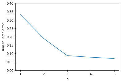
Then, estimate the number of clusters in the data by finding the "elbow" in the graph.
Note: Here is a log to help you debug.
Submission
Link to repl.it code that generates the plot
Github commit to machine-learning repository
In your submission, write down your estimated number of clusters in the data set.
Problem 93
Minimax Strategy Player
a. Implement a minimax player for your tic-tac-toe game.
Remember that the minimax strategy works as follows:
- Create a game tree with all the states of the tic tac toe game
- Identify the nodes that represent terminal states and assign them 1, -1, or 0 depending on whether it corresponds to a win, loss, or tie for you
Repeatedly propogate those scores up the tree to parent nodes.
If the game state of the parent node implies that it's your turn, then the score of that node is the maximum value of the child scores (since you want to maximize your score).
If the game state of the parent node implies that it's the opponent's turn, then the score of that node is the minimum value of the child scores (since your opponent wants to minimize your score).
Remember that we went over the score propagation + implementation recommendations in class, at the end of the computation & modeling portion.
Always make the move that takes you to the highest-score child state. (If there are ties, then you can choose randomly.)
b. Check that your minimax strategy usually beats a random strategy. Run as many minimax vs random matchups as you can in 3 minutes, alternating who goes first. What percentage of the time does minimax win? Post your win percentage on Slack.
Submission
Repl.it link that I can run to simulate & print out your win percentage
Link to github commit (should be a branch of games-cohort-2)
Be ready to present your implementation next week!
Problem 92
Anton & Charlie - Repository Updates
Here is where our shared tic-tac-toe implementation will live:
https://github.com/eurisko-us/games-cohort-2/tree/main/tic-tac-toe
Anton -- create a pull request for your tic-tac-toe implementation, and ping me on Slack once you've made the pull request so that I can accept it. Please do this today (Wednesday) so that Charlie has time to do his part afterwards.
Charlie -- once Anton's game has been pulled in, check that your InputPlayer works with the game implementation, and then create a pull request for your InputPlayer. Let me know once you've made the pull request so that I can accept it.
Game Tree
Construct a game tree for tic-tac-toe. Remember that each node in the game tree corresponds to a state of the game. The root node's state is an empty board. It has 9 children, one for each move that the first player can make. Each of those 9 children have 8 children (after the first player has moved, there are 8 moves remaining for the second player).
This will be similar to a regular Tree class, except that
each node should have a
stateattribute that holds the state of the tic-tac-toe game, aplayerattribute that says whose turn it is, and awinnerattribute that says if someone has won.instead of passing edges into the tree at initialization, you'll need to build up your tree recursively: start with a tree with a single node, and then recursively create child nodes until they reach a terminal state (i.e. a state with a winner).
According to Wikipedia, (https://en.wikipedia.org/wiki/Game_tree#Understanding_the_game_tree), there will be 255,168 leaf nodes. But if you get something different and can't find anything wrong with your code after checking the first couple layers of the tree and the terminal states, let me know and I'll check it out.
Note: On Friday, the assignment will be to create a minimax player and run it against the random player on the shared tic-tac-toe implementation. This assignment is meant to help you get the infrastructure (i.e. game tree) set up to accomplish Friday's assignment.
Submission
Link to your code that generates the game tree. Put this in a branch of the shared repository and submit a link to your branch. Be sure to reach out if you have any issues doing that.
You can call your branch your-name-game-tree.
Problem 91
Clustering
Clustering in General
"Clustering" is the act of finding "groups" of similar records within data.
Watch this video to get a general sense of what clustering is and why we care about it. (Best to play it at 1.5 or 1.75x speed to save time)
K-Means Clustering
Your task will be to implement a basic clustering technique called "k-means clustering". Here is a video describing k-means clustering:
Here is a summary of k-means clustering:
Initialize the clusters
Randomly divide the data into k parts. Each part represents an initial "cluster".
Compute the mean of each part. Each mean represents an initial cluster center.
Update the clusters
Re-assign each record to the cluster with the nearest center (using Euclidean distance).
Compute the new cluster centers by taking the mean of the records in each cluster.
Keep repeating step 2 until the clusters don't change after the update.
Your Task
Write a KMeans clustering class and use it to classify the following data.
# these column labels aren't necessary to use
# in the problem, but they make the problem more
# concrete when you're thinking about what the data
# means.
columns = ['Portion Eggs',
            'Portion Butter',
            'Portion Sugar',
            'Portion Flour']

data = [[0.14, 0.14, 0.28, 0.44],
        [0.22, 0.1, 0.45, 0.33],
        [0.1, 0.19, 0.25, 0.4],
        [0.02, 0.08, 0.43, 0.45],
        [0.16, 0.08, 0.35, 0.3],
        [0.14, 0.17, 0.31, 0.38],
        [0.05, 0.14, 0.35, 0.5],
        [0.1, 0.21, 0.28, 0.44],
        [0.04, 0.08, 0.35, 0.47],
        [0.11, 0.13, 0.28, 0.45],
        [0.0, 0.07, 0.34, 0.65],
        [0.2, 0.05, 0.4, 0.37],
        [0.12, 0.15, 0.33, 0.45],
        [0.25, 0.1, 0.3, 0.35],
        [0.0, 0.1, 0.4, 0.5],
        [0.15, 0.2, 0.3, 0.37],
        [0.0, 0.13, 0.4, 0.49],
        [0.22, 0.07, 0.4, 0.38],
        [0.2, 0.18, 0.3, 0.4]]

# we usually don't know the classes, of the
# data we're trying to cluster, but I'm providing
# them here so that you can actually see that the
# k-means algorithm succeeds.

classes = ['Shortbread',
            'Fortune',
            'Shortbread',
            'Sugar',
            'Fortune',
            'Shortbread',
            'Sugar',
            'Shortbread',
            'Sugar',
            'Shortbread',
            'Sugar',
            'Fortune',
            'Shortbread',
            'Fortune',
            'Sugar',
            'Shortbread',
            'Sugar',
            'Fortune',
            'Shortbread']
Make sure your class passes the following test:
# initial_clusters is a dictionary where the key
# represents the cluster number and the value is
# a list of indices (i.e. row numbers in the data set)
# of records that are said to be in that cluster

>>> initial_clusters = {
    1: [0,3,6,9,12,15,18],
    2: [1,4,7,10,13,16],
    3: [2,5,8,11,14,17]
    }
>>> kmeans = KMeans(initial_clusters, data)
>>> kmeans.run()
>>> kmeans.clusters
{
    1: [0, 2, 5, 7, 9, 12, 15, 18],
    2: [3, 6, 8, 10, 14, 16],
    3: [1, 4, 11, 13, 17]
}
Here are some step-by-step tests to help you along:
>>> initial_clusters = {
    1: [0,3,6,9,12,15,18],
    2: [1,4,7,10,13,16],
    3: [2,5,8,11,14,17]
    }
>>> kmeans = KMeans(initial_clusters, data)

### ITERATION 1
>>> kmeans.update_clusters_once()

>>> kmeans.clusters
{
    1: [0, 3, 6, 9, 12, 15, 18],
    2: [1, 4, 7, 10, 13, 16],
    3: [2, 5, 8, 11, 14, 17]
}
>>> kmeans.centers
{
    1: [0.113, 0.146, 0.324, 0.437],
    2: [0.122, 0.115, 0.353, 0.427],
    3: [0.117, 0.11, 0.352, 0.417]
}
>>> {n: [classes[i] for i in cluster_indices] \
    for cluster_number, cluster_indices in kmeans.clusters.items()}
{
    1: ['Shortbread', 'Sugar', 'Sugar', 'Shortbread', 'Shortbread', 'Shortbread', 'Shortbread'],
    2: ['Fortune', 'Fortune', 'Shortbread', 'Sugar', 'Fortune', 'Sugar'],
    3: ['Shortbread', 'Shortbread', 'Sugar', 'Fortune', 'Sugar', 'Fortune']
}

### ITERATION 2
>>> kmeans.update_clusters_once()

>>> kmeans.clusters
{
    1: [0, 2, 5, 6, 7, 9, 10, 12, 15, 18],
    2: [14, 16],
    3: [1, 3, 4, 8, 11, 13, 17]
}

>>> kmeans.centers
{
    1: [0.111, 0.158, 0.302, 0.448],
    2: [0.0, 0.115, 0.4, 0.495],
    3: [0.159, 0.08, 0.383, 0.379]
}

>>> {n: [classes[i] for i in cluster_indices] \
    for cluster_number, cluster_indices in kmeans.clusters.items()}
{
    1: ['Shortbread', 'Shortbread', 'Shortbread', 'Sugar', 'Shortbread', 'Shortbread', 'Sugar', 'Shortbread', 'Shortbread', 'Shortbread'],
    2: ['Sugar', 'Sugar'],
    3: ['Fortune', 'Sugar', 'Fortune', 'Sugar', 'Fortune', 'Fortune', 'Fortune']
}

### ITERATION 3
>>> kmeans.update_clusters_once()

>>> kmeans.clusters
{
    0: [0, 2, 5, 7, 9, 12, 15, 18],
    1: [3, 6, 8, 10, 14, 16],
    2: [1, 4, 11, 13, 17]
}

>>> kmeans.centers
{
    0: [0.133, 0.171, 0.291, 0.416],
    1: [0.018, 0.1, 0.378, 0.51],
    2: [0.21, 0.08, 0.38, 0.346]
}

>>> {n: [classes[i] for i in cluster_indices] \
    for cluster_number, cluster_indices in kmeans.clusters.items()}
{
    0: ['Shortbread', 'Shortbread', 'Shortbread', 'Shortbread', 'Shortbread', 'Shortbread', 'Shortbread', 'Shortbread'],
    1: ['Sugar', 'Sugar', 'Sugar', 'Sugar', 'Sugar', 'Sugar'],
    2: ['Fortune', 'Fortune', 'Fortune', 'Fortune', 'Fortune']
}
Github
This walkthough has a lot of writing, but it should only take you 10 minutes max to complete it. We did most of it in class.
a. I invited everyone to a team eurisko-us/cohort-2 and gave that team write access to our shared game implementation. Check your email for the invite and accept it.
b. Follow the steps below to practice creating a branch and a pull request.
Our shared game implementation is here:
Here is a high-level guide of the process for making changes to our shared repository:
To clone and enter the repository
>>> git clone https://github.com/eurisko-us/space-empires-cohort-2.git
>>> cd space-empires-cohort-2
To check out a new branch:
>>> git checkout -b justin-comment
Switched to a new branch 'justin-comment'
Add a comment to test.txt (you can just "write YourName was here"). Then, check the status of your branch:
>>> git status
On branch justin-comment
Untracked files:
  (use "git add <file>..." to include in what will be committed)

    test.txt

nothing added to commit but untracked files present (use "git add" to track)
Add your changes and commit to your branch
>>> git add test.txt
>>> git commit -m "create Justin's comment"
[justin-comment 542f30e] create Justin's comment
 1 file changed, 1 insertion(+)
 create mode 100644 justin-comment.txt
Push to your branch
>>> git push origin justin-comment
Username for 'https://github.com': jpskycak
Password for 'https://jpskycak@github.com':
    (for privacy reasons the password won't appear
    as you type it, but your keystrokes will still
    be getting logged, so you just need to type
    your password and press enter)

Counting objects: 3, done.
Delta compression using up to 4 threads.
Compressing objects: 100% (2/2), done.
Writing objects: 100% (3/3), 309 bytes | 309.00 KiB/s, done.
Total 3 (delta 1), reused 0 (delta 0)
remote: Resolving deltas: 100% (1/1), completed with 1 local object.
remote:
remote: Create a pull request for 'justin-comment' on GitHub by visiting:
remote:      https://github.com/eurisko-us/space-empires-cohort-1/pull/new/justin-comment
remote:
To https://github.com/eurisko-us/space-empires-cohort-1.git
 * [new branch]      justin-comment -> justin-comment
On GitHub, it will show that your branch is a commit ahead, and possibly even commits behind (if other people have made commits in the time since you first created your branch).
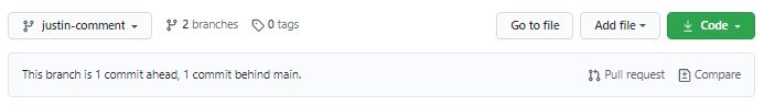
Click "Pull request", and create the pull request. Don't merge it yet, though. We'll do that during the next class.
Submission
Repl.it link to your k-means tests (and your github commit)
Problem 90
Tic-Tac-Toe Game
Create a basic tic-tac-toe game. There should be a Game class that accepts two Player classes, similar to how space-empires works. (You can make additional classes as you see fit.)
You should also include some basic tests to demonstrate that the game works properly. One test to have for sure is to match up two random players against each other, play 100 or 1000 games while alternating who goes first, and then make sure that the players' win rates are roughly equal.
Next class, be ready to present your implementation.
Submission
A link to the tests for your tic-tac-toe implementation
Problem 89
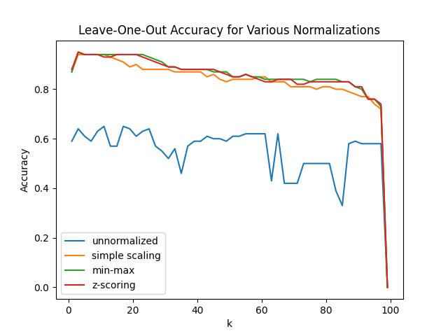
a. Take your code from the previous problem and run it again, this time on the titanic dataset.
Remember that the titanic dataset is provided here:
Filter the above dataset down to the first 100 rows, and only these columns:
["Survived", "Sex", "Pclass", "Fare", "Age","SibSp"]Then, just as before, make a plot of leave-one-out cross validation vs $k$ for k=[1,3,5,7,...,99]. Overlay the 4 resulting plots: "unscaled", "simple scaling", "min-max", "z-score". You should get the following result:
b. Compute the relative speed at which your code runs (relative to mine). The way you can do this is to run this code snippet 5 times and take the average time:
import time
start = time.time()

counter = 0
for _ in range(1000000):
    counter += 1

end = time.time()
print(end - start)
When I do this, I get an average time of about 0.15 seconds. So to find your relative speed, divide your result by mine.
c. Speed up your code in part (a) so it runs in (your relative speed) * 45 seconds or less. I took a deeper dive into some code that was running slow for students, and it turns out the code just needs to be written more efficiently.
To make the code more efficient, you need to avoid unnessarily repeating expensive operations. Anything involving a dataset transformation is usually expensive.
The very first thing you do should be processing all of your data and splitting it into your
Xandyarrays. DON'T do this every time you fit a model -- just do it once at the beginning.In general, avoid repeatedly processing the data set. If there's something you're doing to the data set over and over again, just do it once at the beginning.
You can time your code using the following setup:
import time
begin_time = time.time()

(your code here)

end_time = time.time()
print('time taken:', end_time - start_time)
REALLY IMPORTANT:
While you make your code more efficient, you'll need to repeatedly run it to see if your actions are actually decreasing the time it takes to run. Instead of running the full analysis each time, just run a couple values of $k$. That way, you're not waiting a long time for your code to run each time. Once you've decreased this partial run time by a lot, you can run your entire analysis again.
If you get stuck for more than 10 minutes without making progress, ping me on Slack so that I can take a look at your code and let you know if there's anything else that's making it slow.
d. Complete quiz corrections for any problems you missed. (I'll have the quizzes graded by tonight, 5/5.) That will either involve revising your free response answers or revising your code and sending me the revised version.
Submission
Link to KNN code that runs in (your relative speed) * 45 seconds or less. When I run your code, it should print out the total time it took to run.
Quiz corrections
Problem 88
Before fitting a k-nearest neighbors model, it's common to "normalize" the data so that all the features lie within the same range. Otherwise, variables with larger ranges are given greater distance contributions (which is usually not what we want).
The following video explains 3 different normalization techniques: simple scaling, min-max scaling, and z-scoring.
Consider the following dataset. The goal is to use the features to predict the book type (children's book vs adult book).
First, read in this dataset and change the "book type" column to be numeric (1 if adult book, 0 if children's book).
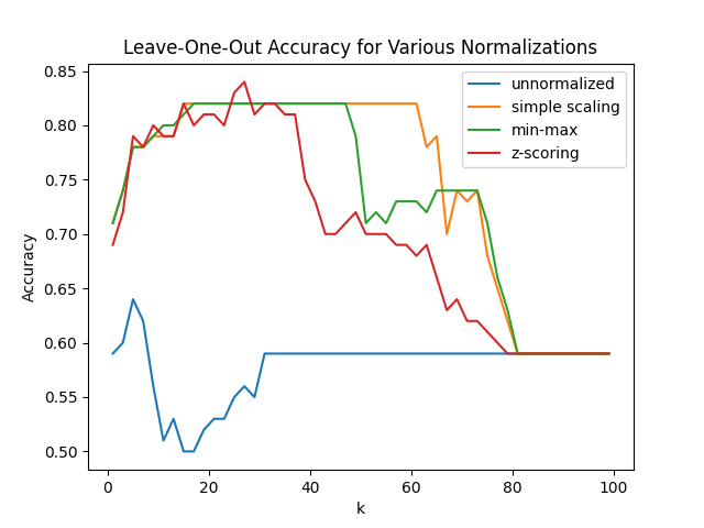
a. Create a "leave-one-out accuracy vs k" curve for k=[1,3,5,...,99].
b. Repeat (a), but this time normalize the data using simple scaling beforehand.
c. Repeat (a), but this time normalize the data using min-max scaling beforehand.
d. Repeat (a), but this time normalize the data using z-scoring beforehand.
e. Overlay all 4 plots on the same graph. Be sure to include a legend that labels the plots as "unscaled", "simple scaling", "min-max", "z-score".
You should get the following result:
f. Answer the big question: why does normalization improve the accuracy? (Or equivalently, why did the model perform worse on the unnormalized data?)
Submission
Overleaf doc with plot and explanation, as well as a link to the code that you wrote to generate the plot.
Problem 87
KNN - Titanic Survival Modeling
Note: Previously, this problem had consisted of a KNN model on the full titanic dataset along with normalization techniques. The analysis was taking too long on chromebooks, so I've reduced the size of the dataset. Also, the normalization techniques weren't having an effect on the result, so I took that off this assignment but will revise the normalization task and put it on the next assignment. Any code you wrote for the normalization techniques will be useful in the next assignment.
In this problem, your task is to use scikit-learn's k-nearest neighbors implementation to predict survival in a portion of the titanic survival modeling dataset.
Remember that the fully-processed dataset is here:
Take that fully-processed dataset and filter it down to the first 100 rows, and only these columns:
[
"Survived",
"Sex",
"Pclass",
"Fare",
"Age",
"SibSp"
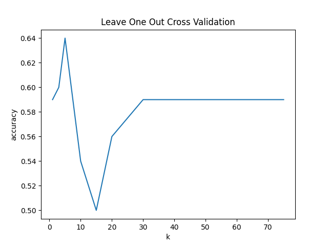
]Then, create a plot of leave-one-out accuracy vs $k$ for the following values of $k{:}$
[1,3,5,10,15,20,30,40,50,75]You should get the following result:
K-Fold Cross Validation
K-fold cross validation is similar to leave-one-out cross validation, except that instead of repeatedly leaving out one record, we split the dataset into $k$ sections or "folds" and repeatedly leave out one of those folds.
This video explains it pretty well, with a really good visual at the end:
Answer the following questions:
If we had a dataset with 800 records and we used 2-fold cross validation, how many models would we fit, how many records would each model be trained on, and how many records would each model be validated (i.e. tested) on?
If we had a dataset with 800 records and we used 8-fold cross validation, how many models would we fit, how many records would each model be trained on, and how many records would each model be validated (i.e. tested) on?
If we had a dataset with 800 records, for what value of $k$ would $k$-fold cross validation be equivalent to leave-one-out cross validation?
Submission
Link to your code that generates the plot
Overleaf doc with the plot and the answers to the 3 questions
Problem 86
K-Nearest Neighbors & Leave-One-Out Cross Validation
Consider the following cookie dataset (it's similar to the one we used before, but it has some additional entries).
>>> df = pd.DataFrame(
    [['Shortbread'  ,     0.14     ,       0.14     ,      0.28     ,     0.44      ],
['Shortbread'  ,     0.10     ,       0.18     ,      0.28     ,     0.44      ],
['Shortbread'  ,     0.12     ,       0.10     ,      0.33     ,     0.45      ],
['Shortbread'  ,     0.10     ,       0.25     ,      0.25     ,     0.40      ],
['Sugar'       ,     0.00     ,       0.10     ,      0.40     ,     0.50      ],
['Sugar'       ,     0.00     ,       0.20     ,      0.40     ,     0.40      ],
['Sugar'       ,     0.02     ,       0.08     ,      0.45     ,     0.45      ],
['Sugar'       ,     0.10     ,       0.15     ,      0.35     ,     0.40      ],
['Sugar'       ,     0.10     ,       0.08     ,      0.35     ,     0.47      ],
['Sugar'       ,     0.00     ,       0.05     ,      0.30     ,     0.65      ],
['Fortune'     ,     0.20     ,       0.00     ,      0.40     ,     0.40      ],
['Fortune'     ,     0.25     ,       0.10     ,      0.30     ,     0.35      ],
['Fortune'     ,     0.22     ,       0.15     ,      0.50     ,     0.13      ],
['Fortune'     ,     0.15     ,       0.20     ,      0.35     ,     0.30      ],
['Fortune'     ,     0.22     ,       0.00     ,      0.40     ,     0.38      ],
['Shortbread'  ,     0.05     ,       0.12     ,      0.28     ,     0.55      ],
['Shortbread'  ,     0.14     ,       0.27     ,      0.31     ,     0.28      ],
['Shortbread'  ,     0.15     ,       0.23     ,      0.30     ,     0.32      ],
['Shortbread'  ,     0.20     ,       0.10     ,      0.30     ,     0.40      ]],
    columns = ['Cookie Type' ,'Portion Eggs','Portion Butter','Portion Sugar','Portion Flour' ]
    )
The goal is to create a k-nearest neighbors model for this data. But there are two issues:
We don't know what value of k to use. Should we use k=2? k=5? k=9? It's not clear.
Our dataset is small (19 data points). If we split it in half for training and validation, we'll be severely handicapping our model's performance (cutting a small dataset in half is usually worse than cutting a big dataset in half) and we might not have enough validation points to draw good conclusions about the performance of the model.
The way to resolve these two issues is to use leave-one-out cross-validation:
For each record in our dataset, we'll train a k-nearest neighbors model on all the OTHER records, and then check whether the model classifies our record correctly.
We'll do this for all records in the data set and compute the accuracy.
Then, we'll plot the accuracy for various values of k and see where it's the highest.
Carry out the above procedure using sklearn's k-nearest neighbors implementation. You should get the following result:
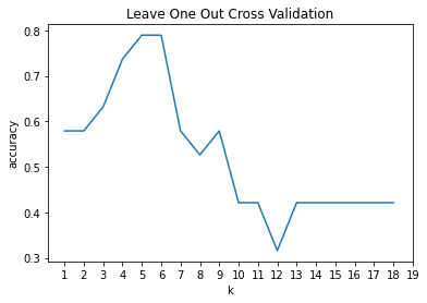
For your debugging purposes, here are the accuracy values you should be getting (rounded to 2 decimal places):
[0.58, 0.58, 0.63, 0.74, 0.79, 0.79, 0.58, 0.53, 0.58, 0.42, 0.42, 0.32, 0.42, 0.42, 0.42, 0.42, 0.42, 0.42]And here is a log:
Once you've got that plot, answer the following questions.
- Why is the accuracy low when k is very low?
- Why is the accuracy low when k is very high?
Submission
Overleaf doc containing your plot and the answers to the 2 questions, along with a commit link to your code that generated the plot.
Remember, quiz Friday! See the previous assignment for information on what's on it.
Problem 85
Space Empires Presentation
Prepare a 3-5 minute presentation about your Space Empires implementation for Wednesday. Don't exceed 5 minutes. Address the following:
- What is your general architecture? E.g. what classes do you use, how does your combat engine work, how is state stored/updated, how do players communicate with the game.
- What are some things your implementation does elegantly?
- What are some things that could be improved, and what kind of state are they in (are they just nice-to-haves, or are there things that will cause major issues down the road if not adjusted)?
You can show parts of your code, but DON'T go through it line-by-line. This is supposed to be a quick elevator pitch of your implementation.
Note: You don't have to make slides or write stuff on notecards or anything like that. You just need to deliver a clear and concise explanation of how your implementation works. But in order to achieve that, you'll need to practice a bit beforehand.
Intro to Minimax Algorithm
To introduce the idea of how one can design intelligent agents, we'll implement an intelligent angent that solves tic-tac-toe using the minimax algorithm. But before we actually implement it, we need to understand it at a high level.
Watch the first 8 minutes of the following video that explains the minimax algorithm. (You can probably set it to 1.5x speed)
Then, answer the following questions:
What does the root of the game tree represent?
What does each edge of the game tree represent?
What are the scores of a win, a loss, a tie? (3 answers)
Is your opponent the maximizing player or the minimizing player?
If a node has a child with score +1 and a child with score -1, then what is the score of the node? Assume it's the opponent's turn.
If a node has two children with score +1, one child with score 0, and one child with score -1, then what is the score of the node? Assume it's the opponent's turn.
Draw the full game tree proceeding from the following root node, and label each node with its score according to the minimax algorithm. There should be 12 nodes in total.
X | O | X
---------
  | O | O
---------
  |   | X
You can do the drawing on paper, take a picture, and put that in your Overleaf doc.
Submission
Overleaf doc with answers to the above questions
Quiz Friday
Forward/backward selection, basic manipulations with pandas / numpy / sklearn.
Problem 84
In this assignment, you'll do "backward selection", which is very similar to forward selection except that we start with all features and remove features that don't improve the accuracy.
One key difference is that with backward selection, we'll just loop through all the features once and remove any features that don't improve the accuracy. This is different from forward selection (in forward selection, we looped through all the features repeatedly).
- The reason why we'll just loop through all the features once is that backward selection is expensive (it takes a long time to fit each model when we're using all the features).
A couple notes:
Use 100 iterations and set
random_state=0(it's a parameter in the logistic regressor; check out the documentation for more info)100 iterations isn't enough for the regressor to converge, but since things run slow on the chromebooks, we'll just do this exercise with 100 iterations regardless. To suppress convergence warnings, set the following:
from warnings import simplefilter
from sklearn.exceptions import ConvergenceWarning
simplefilter("ignore", category=ConvergenceWarning)
Results
Initially, using all the features, testing accuracy should be about 0.788
Then, after backwards selection, testing accuracy should have increased to 0.831
For your ease of debugging, all the features along with information about each iteration of backward selection are shown in the log below.
Problem 83
Quiz Corrections
If there were any problems you didn't get right, fix them and show all your work (or all your code).
Sudoku Solver
Based on feedback about the sudoku puzzle, we'll devote one more assignment to it.
Again, the idea is just a slight extension of the magic square problem (55-1), so if you've forgotten how to do the magic square problem or didn't fully learn it in the first place, then that's the first thing you need to address. I'll be available to field questions on Slack, as always.
Recall this part of the problem statement:
There are 26 open spots, which means there's going to be 26 for loops. That's a lot! It'll be faster if you create a script that writes all these for loops to a separate file, and then you can run that file.
If the idea of writing a script to generate another script threw you off, then ignore it and try writing the 26 loops manually. After a handful of lines you'll notice that you're just doing a repetitive task over and over -- writing a for loop from a basic template and indenting it. Once you get to that point, then you'll be able to see why it'll save you time and headache if you automate the process of writing all these for loops.
Submission
Overleaf doc with quiz corrections, link to sudoku solver on repl.it (it should print out the solution when I run the file).
Problem 82
Location: assignment-problems/sudoku_solver.py
This problem is basically the same as 55-1, except that instead of a magic square, it's a mini sudoku puzzle. The goal is to fill in the grid so that every row, every column, and every 3x2 box contains the digits 1 through 6.
There are 26 open spots, which means there's going to be 26 for loops. That's a lot! It'll be faster if you create a script that writes all these for loops to a separate file, and then you can run that file.
Note: If you need a refresher on the method that we used to solve the magic square, check out Elijah's blog post:
https://www.eurisko.us/solving-magic-squares-using-backtracking/
He managed to consolidate the numerous for loops into a single while loop, which you're free to do if you'd like. But you're not required to use a while loop -- it's okay if you want to just create a script that writes all the for loops to a separate file, and then run that file. (It's not very elegant, but it's just as fast and it gets the job done.)
Lastly: Format your output so that when your code prints out the result, it prints out the result in the shape of a sudoku puzzle:
-----------------
| . . 4 | . . . |
| . . . | 2 3 . |
-----------------
| 3 . . | . 6 . |
| . 6 . | . . 2 |
-----------------
| . 2 1 | . . . |
| . . . | 5 . . |
-----------------
Make sure to look at your solution to check that it is indeed correct!
Problem 81
Note: Initially, I was hoping to write a problem involving space empires development, but I need some more time to put one together (to ensure the problem doesn't take too long). So, here's a problem that involves implementing one of the simplest machine learning models, the "k-nearest neighbors" model.
Libraries: Feel free to use pandas and numpy. But NOT sklearn. You need to implement this model on your own, not just import it from sklearn. But you can use pandas dataframes and numpy arrays to help you.
The dataset below displays the ratio of ingredients for various cookie recipes.
>>> df = pd.DataFrame(
    [['Shortbread'  ,     0.14     ,       0.14     ,      0.28     ,     0.44      ],
    ['Shortbread'  ,     0.10     ,       0.18     ,      0.28     ,     0.44      ],
    ['Shortbread'  ,     0.12     ,       0.10     ,      0.33     ,     0.45      ],
    ['Shortbread'  ,     0.10     ,       0.25     ,      0.25     ,     0.40      ],
    ['Sugar'       ,     0.00     ,       0.10     ,      0.40     ,     0.50      ],
    ['Sugar'       ,     0.00     ,       0.20     ,      0.40     ,     0.40      ],
    ['Sugar'       ,     0.10     ,       0.08     ,      0.35     ,     0.47      ],
    ['Sugar'       ,     0.00     ,       0.05     ,      0.30     ,     0.65      ],
    ['Fortune'     ,     0.20     ,       0.00     ,      0.40     ,     0.40      ],
    ['Fortune'     ,     0.25     ,       0.10     ,      0.30     ,     0.35      ],
    ['Fortune'     ,     0.22     ,       0.15     ,      0.50     ,     0.13      ],
    ['Fortune'     ,     0.15     ,       0.20     ,      0.35     ,     0.30      ],
    ['Fortune'     ,     0.22     ,       0.00     ,      0.40     ,     0.38      ]],
    columns = ['Cookie Type' ,'Portion Eggs','Portion Butter','Portion Sugar','Portion Flour' ]
    )
Suppose you're given a cookie recipe and you want to determine whether it is a shortbread cookie, a sugar cookie, or a fortune cookie. The cookie recipe consists of
0.10 portion eggs,
0.15 portion butter,
0.30 portion sugar, and
0.45 portion flour.
We will infer the classification of this cookie using the $k$ nearest neighbors approach. Here is an illustration of the approach using $k=5.$
We represent the cookie as the point $P(0.10, 0.15, 0.30, 0.45).$
We compute the Euclidean distance $$ d(a,b) = \sqrt{ (a_1-b_1)^2 + (a_2-b_2)^2 + \cdots + (a_n - b_n)^2} $$ between $P$ and each of the points corresponding to cookies in the dataset. In this case, the distances are as follows:
['Distance', 'Cookie Type' ,'Portion Eggs','Portion Butter','Portion Sugar','Portion Flour' ]
[[0.047    , 'Shortbread'  ,     0.14     ,       0.14     ,      0.28     ,     0.44      ],
[0.037    , 'Shortbread'  ,     0.10     ,       0.18     ,      0.28     ,     0.44      ],
[0.062    , 'Shortbread'  ,     0.12     ,       0.10     ,      0.33     ,     0.45      ],
[0.123    , 'Shortbread'  ,     0.10     ,       0.25     ,      0.25     ,     0.40      ],
[0.158    , 'Sugar'       ,     0.00     ,       0.10     ,      0.40     ,     0.50      ],
[0.158    , 'Sugar'       ,     0.00     ,       0.20     ,      0.40     ,     0.40      ],
[0.088    , 'Sugar'       ,     0.10     ,       0.08     ,      0.35     ,     0.47      ],
[0.245    , 'Sugar'       ,     0.00     ,       0.05     ,      0.30     ,     0.65      ],
[0.212    , 'Fortune'     ,     0.20     ,       0.00     ,      0.40     ,     0.40      ],
[0.187    , 'Fortune'     ,     0.25     ,       0.10     ,      0.30     ,     0.35      ],
[0.396    , 'Fortune'     ,     0.22     ,       0.15     ,      0.50     ,     0.13      ],
[0.173    , 'Fortune'     ,     0.15     ,       0.20     ,      0.35     ,     0.30      ],
[0.228    , 'Fortune'     ,     0.22     ,       0.00     ,      0.40     ,     0.38      ]],
We consider the 5 points that are closest to $P.$ (These are the 5 "nearest neighbors".)
['Shortbread', 0.037]
['Shortbread', 0.047]
['Shortbread', 0.062]
['Sugar', 0.088]
['Shortbread', 0.123]
We predict the majority class, which in this case happens to be
Shortbread. (If there is a tie, then we predict the class with the lower average distance.)
Watch this 2-minute video on kNN to really drive the idea home: https://www.youtube.com/watch?v=0p0o5cmgLdE
Your task is to create a class KNearestNeighborsClassifier that works as follows.
>>> knn = KNearestNeighborsClassifier(k=5)
>>> knn.fit(df, dependent_variable = 'Cookie Type')
>>> observation = {
    'Portion Eggs': 0.10,
    'Portion Butter': 0.15,
    'Portion Sugar': 0.30,
    'Portion Flour': 0.45
}

>>> knn.compute_distances(observation)
Returns a dataframe representation of the following array:

[[0.047, 'Shortbread'],
 [0.037, 'Shortbread'],
 [0.062, 'Shortbread'],
 [0.122, 'Shortbread'],
 [0.158, 'Sugar'],
 [0.158, 'Sugar'],
 [0.088, 'Sugar'],
 [0.245, 'Sugar'],
 [0.212, 'Fortune'],
 [0.187, 'Fortune'],
 [0.396, 'Fortune'],
 [0.173, 'Fortune'],
 [0.228, 'Fortune']]

Note: the above has been rounded to 3 decimal places for ease of viewing, but you should not round in your
actual class.

>>> knn.nearest_neighbors(observation)
Returns a dataframe representation of the following array:

[[0.037, 'Shortbread'],
 [0.047, 'Shortbread'],
 [0.062, 'Shortbread'],
 [0.088, 'Sugar'],
 [0.122, 'Shortbread'],
 [0.158, 'Sugar'],
 [0.158, 'Sugar'],
 [0.173, 'Fortune'],
 [0.187, 'Fortune'],
 [0.212, 'Fortune'],
 [0.228, 'Fortune'],
 [0.245, 'Sugar'],
 [0.396, 'Fortune']]

>>> knn.classify(observation)
'Shortbread' # because this is the majority class
             # in the 5 nearest neighbors
Remember that in the case of a tie, you need to chose whichever class has a lower average distance (where only the first k entries are considered in the average).
Here is a test to make sure you've implemented that properly:
df = pd.DataFrame(
    [['A', 0],
     ['A', 1],
     ['B', 2],
     ['B', 3]],
     columns = ['letter', 'number']
)

>>> knn = KNearestNeighborsClassifier(k=4)
>>> knn.fit(df, dependent_variable = 'letter')
>>> observation = {
    'number': 1.6
}
>>> knn.classify(observation)
'B'
Submission: Links to your repl.it files:
machine-learning/src/k_nearest_neighbors_classifier.py
machine-learning/tests/test_k_nearest_neighbors_classifier.py
Also, the commit link to your machine-learning repository.
Problem 80
Previously, you built a logistic model with 167 features, and got the following results using max_iter=10,000:
training: 0.848
testing: 0.811
It turned out that running that many iterations was taking a while (5 minutes) for some students, so let's use max_iter=1,000 instead. The logistic regressor might not fully converge, which means the model will probably be slightly worse, but that's okay because right now just going through this modeling process for educational purposes.
Using max_iter=1,000, I get the following results:
training: 0.846
testing: 0.808
Yours should be pretty similar.
Now, you'll notice that the training accuracy is quite a bit higher than the testing accuracy. This is because we now have a LOT of features in our dataset, and not all of them are useful, which means it's harder for the model to figure out what is useful. The model ends up fitting to some "noise" in the data (see https://en.wikipedia.org/wiki/Noisy_data) and that causes it to pick up on some random patterns that aren't actually meaningful. The model becomes paranoid!
To fix this issue, we need to carry out feature selection, in which we attempt to select only the features that are actually useful to the model.
One type of feature selection method is forward selection, in which we begin with an empty model and add in variables one by one. In each forward step, you add the one variable that gives the single best improvement to your model.
Your task is to carry out forward selection on those 167 features.
Initially, you'll assume a model with no features. You don't actually build this model, but you assume its accuracy is 0.
Each forward step, you'll need to create a new model for each possible feature you might add next.
The next feature should always be the feature that gives you the largest accuracy when included in your model.
- If there are any ties, you can just use the feature that you checked first. That way, you'll be able to compare to the log I provide at the bottom of the assignment.
Stopping Criterion: If the feature that gives the largest accuracy doesn't actually improve the accuracy of the model, then stop.
In general, in the $n$th step of forward selection, you should be testing out models with $n$ features, $n-1$ of which are the same across all the models.
Put this problem in a separate file. I'll give you the processed data set so that you can be sure you're using the right starting point (it should match up with yours, but just in case it doesn't you can still do this problem without having to go down the rabbit hole of debuggin your data processing).
Your task is to take the processed data set and carry out forward selection. You should end up with the features and accuracies shown below.
['Sex', 'Pclass * SibSp', 'Pclass * Fare', 'Pclass * CabinType=E', 'Fare * CabinType=D', 'SibSp * CabinType=B', 'SibSp>0', 'Fare * CabinType=A']
training: 0.818
testing: 0.806
Print out a log like that given in the file below. This log is given to help you debug.
IMPORTANT: While initially writing your code, change max_iter to a small number like 10 so that you're not waiting around for your log to generate each time. Once your code seems like it's working as intended, THEN update the iterations to 1000 and check that your results match up with those given in the log above.
You'll notice that we were able to remove a TON of the features, and get nearly the same testing accuracy. The training accuracy also got closer to the testing accuracy. That's good.
However, the testing accuracy didn't increase. It actually went down a bit. In a future assignment, we'll talk about another feature selection method that solves this issue.
Submission
Just the repl.it link to your file and the commit link for Qithub.
Also, remember that there's a quiz on Friday (as outlined on the previous assignment).
Problem 79
Titanic Survival Prediction - Interaction Features
Put your code for this problem in the file that you've been using to do the titanic survival prediction using pandas, numpy, and sklearn.
Previously, we left off using a logistic regression with the following features:
['Sex', 'Pclass', 'Fare', 'Age', 'SibSp', 'SibSp>0', 'Parch>0', 'Embarked=C', 'Embarked=None', 'Embarked=Q', 'Embarked=S', 'CabinType=A', 'CabinType=B', 'CabinType=C', 'CabinType=D', 'CabinType=E', 'CabinType=F', 'CabinType=G', 'CabinType=None', 'CabinType=T']We got the following accuracy:
training accuracy: 0.8260
testing accuracy: 0.7903
Now, let's introduce some interaction terms. You'll need to create another column for each non-redundant interaction between features. An interaction is redundant if the two features are derived from the same original feature.
SibSpandSibSp>0are redundantAll the features that start with
Embarked=are redundant with each otherAll the features that start with
CabinType=are redundant with each other
I can't give you a list of all these features because then you could just copy over that list and use it as a starting point. But I can tell you that there will be 167 features in total, not including Survival (which is not actually a feature since that's what we're trying to predict). There are 20 non-interaction features and 147 interaction features for a total of 167 features.
There are many ways to accomplish this. My suggestion is to first just create a list of all the names of interaction terms between non-redundant features,
['Sex * Pclass', 'Sex * Fare', ...]and then loop through that list to create the actual column in your dataframe for each interaction feature.
If you fit your regressor using all 167 features with max_iterations=10000, you should get the following result (rounded to 3 decimal places)
training: 0.848
testing: 0.811
Note that at this point, our model is probably overfitting a bit. In a future assignment, we'll fix that by introducing some basic "feature selection" methods.
Submission
Just submit the repl.it link to your file along with the Github commit to your kaggle repository. Your file should print out your training and testing accuracy, which should match up with the given result.
Quiz
We'll have a quiz on Friday on the following topics:
logistic regression (pseudoinverse & gradient descent)
basic data processing / model fitting with pandas / numpy / sklearn
Note that in class today, we reviewed the logistic regression part, but the questions I ask on the quiz aren't going to be exactly the same as the ones we went over in the review. The quiz will check whether you've developed intuition from really understanding the answers to those questions, and the intuition should carry over to similar but slightly different questions.
I may ask you to do some computations by hand, so make sure you're able to do that too (I'd suggest to work out the first iteration in problem 76 by hand and make sure that the gradient & updated weights you get match up with what's in the log).
Problem 78
a. Resolve all my comments (in blue) in your blog posts.
(Justin & Cayden -- you guys don't have comments, since you've been keeping up with your blog posts 100%.)
Once you've resolved the comments, you'll be done with the first draft of your blog post. After break, we'll pass around the blog posts for review and then we'll finalize them.
b. When we post the blog posts, there will be a little "about the author" section at the end. So, submit a bio AND a headshot that you want to be included on the website: https://eurisko.us/people/
Don't worry about cropping or removing the background from the headshot. I'll take care of all of that.
Problem 77
(This is a short ~30 minute assignment since we have Wednesday off.)
Now that you've built a logistic regressor that uses gradient descent, you've "unlocked" the privilege to use sklearn's LogisticRegressor.
Previously, you carried out a Titanic prediction problem using sklearn's linear regressor. For this problem, just tweak the code you wrote to use the logistic regressor instead.
After you replace LinearRegressor with LogisticRegressor in your code, you'll have to
tweak a parameter of the regressor to get it to run long enough to converge
update your code to support the format in which the logistic regressor returns information
I'm not going to tell you exactly how to fix those issues, because the point of this problem is to give you practice debugging and reading documentation.
Tip: To find the official documentation on sklearn's logistic regressor, do a google search with the query "sklearn logistic regression".
You should get the output below. The predictions with the logistic regressor turn out to be a little bit better than those with the linear regressor.
features: [
    'Sex',
    'Pclass',
    'Fare',
    'Age',
    'SibSp', 'SibSp>0',
    'Parch>0',
    'Embarked=C', 'Embarked=None', 'Embarked=Q', 'Embarked=S',
    'CabinType=A', 'CabinType=B', 'CabinType=C', 'CabinType=D', 'CabinType=E', 'CabinType=F', 'CabinType=G', 'CabinType=None', 'CabinType=T']

training accuracy: 0.8260
testing accuracy: 0.7903

coefficients:
{
    'Constant': 1.894,
    'Sex': 2.5874,
    'Pclass': -0.6511,
    'Fare': -0.0001,
    'Age': -0.0398,
    'SibSp': -0.545,
    'SibSp>0': 0.4958,
    'Parch>0': 0.0499,
    'Embarked=C': -0.2078, 'Embarked=None': 0.0867, 'Embarked=Q': 0.479, 'Embarked=S': -0.3519,
    'CabinType=A': -0.0498, 'CabinType=B': 0.0732, 'CabinType=C': -0.2125, 'CabinType=D': 0.7214, 'CabinType=E': 0.4258, 'CabinType=F': 0.6531, 'CabinType=G': -0.7694, 'CabinType=None': -0.5863, 'CabinType=T': -0.2496
}
Submission Template
Just submit the repl.it link to your code. When I run it, it should print out the information above.
Problem 76
Refresher
Previously, we built a LogisticRegressor that worked by reducing the regression task down to the task of finding the least-squares solution to a linear system.
More precisely, the task of fitting the logistic function
$$y=\dfrac{1}{1+e^{\beta_0 + \beta_1 x_1 + \cdots + \beta_n x_n}}$$was reduced to the task of fitting the linear regression
$$\beta_0 + \beta_1 x_1 + \cdots + \beta_n x_n = \ln \left( \dfrac{1}{y} - 1 \right).$$Issue with LogisticRegressor
Although this is a slick way to solve the problem, it suffers from the fact that we have to do something "hacky" in order to fit any data points with $y=0$ or $y=1.$
In such cases, we can't just run the model as usual, because the $\ln \left( \dfrac{1}{y}-1 \right)$ term blows up -- so our "hack" has been to
change any instances of $y=0$ to a small decimal like $y=0.1$ or $y=0.001,$ and
change any instances of $y=1$ to $1$ minus the small decimal, like $y=0.9$ or $y=0.999,$
depending on the context of the problem.
But this isn't a great way to deal with the issue, because the resulting logistic function can change significantly depending on what small decimal we use. The difference between small decimals may seem like such a minor difference, but when we plug these values in the $\ln \left( \dfrac{1}{y} - 1 \right)$ term, we get wildly different results, which leads to quite different fits.
PART A. To illustrate the quite different fits, fit 4 instances of your current LogisticRegressor to the following dataset:
one instance where you change all instances of
y=0toy=0.1and all instances ofy=1toy=0.9another instance where you change all instances of
y=0toy=0.01and all instances ofy=1toy=0.99another instance where you change all instances of
y=0toy=0.001and all instances ofy=1toy=0.999another instance where you change all instances of
y=0toy=0.0001and all instances ofy=1toy=0.9999
df = DataFrame(
    [[1,0],
    [2,0],
    [3,0],
    [2,1],
    [3,1],
    [4,1]],
    columns = ['x', 'y'])
Put these all on the same plot, along with the data, and put them in an Overleaf doc. Be sure to label each curve with 0.1, 0.01, 0.001, or 0.0001 as appropriate.
If you need a refresher on plotting / labeling curves, see here:
https://www.eurisko.us/files/assignment_problems_cohort_2_10th.html#Problem-10-1
If you need a refresher on including data in plots, see here:
https://www.eurisko.us/files/assignment_problems_cohort_2_10th.html#Problem-33-1
Explain: How does the plot change as the small decimal is varied?
Gradient Descent to the Rescue
Instead, we can use gradient descent to fit our logistic function. We want to choose the coefficients that minimize the sum of squared error (the RSS).
PART B. In your LogisticRegressor class, write the following methods:
calc_rss()- calculates the sum of squared error for the regressorset_coefficients(coeffs)- allows you to manually set the coefficients of your regressor by passing in a dictionary of coefficientscalc_gradient(delta)- computes the partial derivatives of the RSS with respect to each coefficientgradient_descent(alpha, delta, num_steps, debug_mode=False)- carries out a given number of steps of gradient descent. Ifdebug_mode=True, then print out every step of the way.
Note that we wrote a gradient descent optimizer that a while back:
https://www.eurisko.us/files/assignment_problems_cohort_2_10th.html#Problem-34-2
You can use this as a refresher on how to code up gradient descent, and you might be able to copy/paste some code from here.
- Unfortunately, you can't just pass your logistic regressor into this gradient descent optimizer class -- we wrote optimizer to work on functions whose parameters were passed in as individual arguments, whereas our
LogisticRegressorstores its coefficients in a dictionary.
Note that we will use the central difference approximation
$$ f'(x) \approx \dfrac{f(x+\delta) - f(x-\delta)}{2\delta}. $$Here is a test case:
df = DataFrame.from_array(
    [[1,0],
    [2,0],
    [3,0],
    [2,1],
    [3,1],
    [4,1]],
    columns = ['x', 'y'])

reg = LogisticRegressor(df, dependent_variable='y')

reg.set_coefficients({'constant': 0.5, 'x': 0.5})

alpha = 0.01
delta = 0.01
num_steps = 20000
reg.calc_gradient(alpha, delta, num_steps)

reg.coefficients

{'constant': 2.7911, 'x': -1.1165}
Here are logs for every step of the way:
Make a plot of the resulting logistic curve, along with the data, and put it in an Overleaf doc.Be sure to label your curve with "gradient descent".
Submission Template
link to Overleaf doc (just contains 2 plots and the explanation of the first plot): ____
repl.it link to code that generated the plots: _____
commit link (machine-learning): ____
Problem 75
Going forward, we need to to start using models from an external machine learning library after you build the initial versions of the corresponding models. Most of the learning comes from building the first version, and debugging these subtle issues takes up too much time. Plus, it's good to know how to work with external libraries.
So instead of "build everything from scratch and maintain it forever", our motto will be "build the first version from scratch and then switch to a popular library".
Important Note
If you're behind on any machine learning problems, don't worry about catching up. Just start off with this problem. This problem doesn't depend on anything you've written previously.
The Problem
Create a new repository called kaggle. Create a folder titanic, and put your dataset and analysis file in there. Remember that the dataset is here:
In this assignment, you will create an analysis.py file that carries out an analysis similar to that described in problem 107, using the libraries numpy, pandas, and sklearn. You should follow along with the relevant parts of the walkthrough in the class recording:
Here are the relevant parts. (But read the rest of the assignment before starting.)
[0:35-0:42] Set up the environment & read in the dataframe
[0:42-0:50] Process
Sexby changingmaleto0andfemaleto1[0:56-1:02] Process
Ageby replacing allNaNs with the mean age[1:02-1:09] Process
SibSpandParch. KeepSibSp, but also add the indicator variable (i.e. dummy variable)SibSp>0. Add the indicator variableParch>0as well, and get rid ofParch.[1:17-1:42] Split into train/test, fit the regressor, get the predictions, compute training/testing accuracy. (At this point, don't worry about checking your numbers match up with mine, since I wasn't showing exactly which columns were being used in the regressor.)
[1:42-1:46] State the columns to be used in the regressor. (Here, your numbers should match up with mine, since I show exactly which columns are being used in the regressor.)
[1:46-1:56] Process
CabinintoCabinTypeand create the corresponding indicator variables. Also, create the corresponding indicator variables forEmbarked. Make sure to deleteCabin,CabinType, andEmbarkedafterwards.[2:00-2:02] Run the final model. Your numbers should match up with mine.
You can just follow along with the walkthrough in the class recording and turn in the code you write as you followed along.
Note that watching me type and speak at normal (slow) pace is a waste of time, so play the video on 2x speed. You can access the speed controls by clicking on the gear icon in the bottom-right of the video.
I think this is a 90-minute problem. The relevant parts of the recording take up 70 minutes, and if you play at 2x speed, it's only 35 minutes. If we budget an equal or double time for you to write the code as you follow along, then we're up to 90 minutes. But if you find yourself taking longer or getting stuck anywhere, please let me know.
Here is the documentation for LinearRegressor():
https://scikit-learn.org/stable/modules/generated/sklearn.linear_model.LinearRegression.html
At the end, your code should print out the following (where numbers are rounded to 4 decimal places):
features: [
    'Sex',
    'Pclass',
    'Fare',
    'Age',
    'SibSp', 'SibSp>0',
    'Parch>0',
    'Embarked=C', 'Embarked=None', 'Embarked=Q', 'Embarked=S',
    'CabinType=A', 'CabinType=B', 'CabinType=C', 'CabinType=D', 'CabinType=E', 'CabinType=F', 'CabinType=G', 'CabinType=None', 'CabinType=T']

training accuracy: 0.81
testing accuracy: 0.7749

coefficients:
{
    'Constant': 0.696,
    'Sex': 0.5283,
    'Pclass': -0.0978,
    'Fare': 0.0,
    'Age': -0.0058,
    'SibSp': -0.0585, 'SibSp>0': 0.0422,
    'Parch>0': 0.0097,
    'Embarked=C': -0.0547, 'Embarked=None': 0.052, 'Embarked=Q': 0.0709, 'Embarked=S': -0.0682,
    'CabinType=A': 0.0447, 'CabinType=B': 0.0371, 'CabinType=C': -0.0124, 'CabinType=D': 0.1818, 'CabinType=E': 0.1088, 'CabinType=F': 0.2593, 'CabinType=G': -0.2797, 'CabinType=None': -0.0677, 'CabinType=T': -0.2717
}
Submission Template:
Just submit 2 things:
- the repl.it link to
kaggle/titanic/analysis.py - the link to your github commit
Problem 74
Announcement
We're going to cut down on Eurisko assignment durations by a third. We've made a lot of progress, and most of you have AP tests coming up, so we're going to ease off the gas pedal a bit. We're going to hit the brakes on Haskell, C++, and code review, since you've had some basic exposure to those things and pursuing them further isn't going to be as valuable to the goals of the class as the space empires and machine learning stuff. Each assignment will consist of a single problem in one of the following areas:
- implementing something in space empires
- implementing part of a machine learning model
- implementing part of a data structure (e.g. Matrix, DataFrame)
- prepping/exploring some data for modeling
- carrying out a model and interpreting the results
- writeups (such as blog posts)
Titanic Survival Modeling
For this problem, you'll need to turn in both your analysis code and an Overleaf writeup. The code should print out all the checks that are provided to you in this problem.
Note: after this problem was released, I realized I forgot to include a Constant column, as we should normally do for linear regression. However, the main things to be learned on this assignment don't really depend on the constant, so carry on without it.
a. Continue processing your data as follows:
Sex- replace"male"with0and"female"with1Age- replace any instances ofNonewith the mean age (which should be about29.699)SibSp- this was one of the variables that didn't have a clear positive or negative association withSurvival. WhenSibSp=0, the survival was low; whenSibSp>=1, the survival started higher but then decreased asSibSpdecreased.So, what we can do is create a dummy variable
SibSp=0that equals1whenSibSpis equal to0(and0otherwise). And we'll keepSibSpas well. This way, the variableSibSp=0can be given a negative coefficient that offsets the coefficient ofSibSpin the case whenSibSpequals0.Parch- we'll replace this with a dummy variableParch=0, because the only significant difference in the data is whether or notParchis equal to0. Among passengers who hadParchgreater than0, it doesn't look like there's much variation in survival.CabinType- replace this with dummy variables of the formCabinType=A,CabinType=B,CabinType=C,CabinType=D,CabinType=E,CabinType=F,CabinType=G,CabinType=None,CabinType=T.Embarked- replace this with dummy variables of the formEmbarked=C,Embarked=None,Embarked=Q,Embarked=S.
Now, your data should all be numeric, and we can put it into linear regressor.
Note: To get predictions out of the linear regressor, we'll interpret the linear regression's output in the following way.
if the linear regressor predicts a value less than
0.5, then it predicts the passenger did not survived (i.e. it predictssurvival=0)if the linear regressor predicts a value greater than or equal to
0.5, then it predicts the passenger survived (i.e. it predictssurvival=1)
b. Create train and test datasets. Use first 500 records for training, and the rest for testing. Start out just training a model which uses Sex as the only feature. This will be our baseline.
train accuracy: 0.8
test accuracy:  0.7698

{'Sex': 0.7420}
Note that accuracy is just the number of correct classifications divided by the total number of classifications.
c. Now, introduce Pclass. Uh oh! Why didn't our test accuracy get any better? Write your explanation in an Overleaf doc.
train accuracy: 0.8
test accuracy:  0.7698

{'Sex': 0.6514, 'Pclass': 0.0419}
Hint: Look at the Sex coefficient.
d. Bring in some more features: Fare, Age, SibSp, SibSp=0, Parch=0. The test accuracy still hasn't gotten any better. Why?
train accuracy: 0.796
test accuracy:  0.7698

{
    'Sex': 0.5833,
    'Pclass': -0.0123,
    'Fare': 0.0012,
    'Age': 0.0008,
    'SibSp': -0.0152,
    'SibSp=0': 0.0478,
    'Parch=0': 0.0962
}
e. Bring in some more features: Embarked=C, Embarked=None, Embarked=Q, Embarked=S. Now the model actually got better. Why is the model more accurate now?
train accuracy: 0.806
test accuracy:  0.7902813299232737

{
    'Sex': 0.4862,
    'Pclass': -0.1684,
    'Fare': 0.0002,
    'Age': -0.0056,
    'SibSp': -0.0719,
    'SibSp=0': -0.0784,
    'Parch=0': -0.0269,
    'Embarked=C': 0.9179,
    'Embarked=None': 1.0522,
    'Embarked=Q': 0.9282,
    'Embarked=S': 0.8544
}
f. Bring in some more features: CabinType=A, CabinType=B, CabinType=C, CabinType=D, CabinType=E, CabinType=F, CabinType=G, CabinType=None. The model is continuing to get better.
train accuracy: 0.816
test accuracy:  0.8005

{
    'Sex': 0.4840,
    'Pclass': -0.1313,
    'Fare': 0.0003,
    'Age': -0.0058,
    'SibSp': -0.0724,
    'SibSp=0': -0.0823,
    'Parch=0': -0.0187,
    'Embarked=C': 0.5446,
    'Embarked=None': 0.6773,
    'Embarked=Q': 0.5522,
    'Embarked=S': 0.4829,
    'CabinType=A': 0.3830,
    'CabinType=B': 0.3360,
    'CabinType=C': 0.2686,
    'CabinType=D': 0.4311,
    'CabinType=E': 0.4973,
    'CabinType=F': 0.4679,
    'CabinType=G': 0.0858,
    'CabinType=None': 0.2634
}
g. Now, introduce CabinType=T. You'll probably see the accuracy go down. I won't include a check because different people will get different results for this one. Why did the accuracy go down?
This is subtle, so I'll give a hint. Look at the entries of $X^TX$ and compare to what the entries looked like before you introduced CabinType=T. The entries get extremely large/small.
So, there are really two questions:
- Why are the extremely large/small entries of $(X^TX)^{-1}$ leading to lower classification accuracy?
- (Harder) Why are the entries of $(X^TX)^{-1}$ getting extremely large/small in the first place?
Submission Template
For your submission, copy and paste your links into the following template:
overleaf link to explanations: _____

repl.it link to file that prints out
the results of your model (it should
match up with the checks in the
assignment): _____

commit link (machine-learning): ____
Problem 73-1
In the Titanic dataset, let's get a sense of how the continuous variables (Age and Fare) relate to Survived.
a. For Age, filter the records down to age categories (0-10, 10-20, 20-30, ..., 70-80) and compute the survival rate (i.e. mean survival) in each category. Exclude any Nones from the analysis.
Put a table in an overleaf document. Round the survival rate to $2$ decimal places (otherwise it's difficult to read.)
In the table, include the counts in parentheses. So each table entry should look like
survivalRate (count). So if the survival rate were0.13and the count were27people, then you'd put0.13 (27).What does the table tell you about the relationship between age and survival?
Give a plausible explanation for why this is.
b. For Fare, filter the records down to fare categories (0-5, 5-10, 10-20, 20-50, 50-100, 100-200, 200+) and compute the survival rate (i.e. mean survival) in each category. Exclude any Nones from the analysis.
- Put a table in the overleaf document and answer the same questions that you did for part (a).
Problem 73-2
SQL Parser
Update your query method to support ORDER BY. The query
df.query("SELECT selectColname1, selectColname2, selectColname3 ORDER BY orderColname1 order1, orderColname2 order2, orderColname3 order3")should be parsed and read into the following primitive operations:
df.order_by(orderColname3, order3)
  .order_by(orderColname2, order2)
  .order_by(orderColname1, order1)
  .select([selectColname1, selectColname2, selectColname3])
Assert that your method passes the following tests:
>>> df = DataFrame.from_array(
    [['Kevin', 'Fray', 5],
    ['Charles', 'Trapp', 17],
    ['Anna', 'Smith', 13],
    ['Sylvia', 'Mendez', 9]],
    columns = ['firstname', 'lastname', 'age']
)

>>> df.query("SELECT lastname, firstname, age ORDER BY age DESC").to_array()
[['Trapp', 'Charles', 17],
['Smith', 'Anna', 13],
['Mendez', 'Sylvia', 9],
['Fray', 'Kevin', 5]]

>>> df.query("SELECT firstname ORDER BY lastname ASC").to_array()
[['Kevin'],
['Sylvia'],
['Anna'],
['Charles']]
Assert that your method passes these tests as well:
>>> df = DataFrame.from_array(
    [['Kevin', 'Fray', 5],
    ['Melvin', 'Fray', 5],
    ['Charles', 'Trapp', 17],
    ['Carl', 'Trapp', 17],
    ['Anna', 'Smith', 13],
    ['Hannah', 'Smith', 13],
    ['Sylvia', 'Mendez', 9],
    ['Cynthia', 'Mendez', 9]],
    columns = ['firstname', 'lastname', 'age']
)

>>> df.query("SELECT lastname, firstname, age ORDER BY age ASC, firstname DESC").to_array()
[['Fray', 'Melvin', 5],
['Fray', 'Kevin', 5],
['Mendez', 'Sylvia', 9],
['Mendez', 'Cynthia', 9],
['Smith', 'Hannah', 13],
['Smith', 'Anna', 13],
['Trapp', 'Charles', 17],
['Trapp', 'Carl', 17]]
Problem 73-3
Commit + Review
Commit your code to Github.
Resolve 1 GitHub issue on one of your own repositories. (If you don't have any issues to resolve, just write a note in your submission that that's the case.)
Submission Template
For your submission, copy and paste your links into the following template:
overleaf link to titanic analysis: _____
repl.it link to sql parser: _____

link to resolved issue: ____
Commit links (machine-learning): ____
Problem 72-1
This will be a "consolidation problem." Your task is to make sure that you have Problem 71-1 completed by the end of the weekend.
Problem 72-2
Quiz Corrections
Correct any errors on your quiz (if you got a score under 100%). You can just submit corrected code and/or explanations (you don't have to explain why you got it wrong in the first place).
Remember that we went through the quiz during class, so if you have any questions or need any help, look at the recording first.
C++
Write a C++ program that creates an array {11, 12, 13, 14} and prints out the memory address of the array and of each element.
Format your output like this:
array has address 0x7fff58f44160
index 0 has value 11 and address 0x7fff58f44160
index 1 has value 12 and address 0x7fff58f44164
index 2 has value 13 and address 0x7fff58f44168
index 3 has value 14 and address 0x7fff58f4416c
Note that your memory addresses will not be the same as those above. (Each time you run the program, the memory addresses will be different.)
Note: If you're having trouble figuring out where to start, remember that we've answered conceptual questions about pointers and the syntax of pointers using this resource:
https://www.learncpp.com/cpp-tutorial/introduction-to-pointers/
Problem 72-3
Commit + Review
Commit your code to Github.
Resolve 1 GitHub issue on one of your own repositories. (If you don't have any issues to resolve, just write a note in your submission that that's the case.)
Submission Template
For your submission, copy and paste your links into the following template:
link to diff that says your log matches up with the given log: _____
link to quiz corrections (if applicable): _____
link to c++ problem: _____

link to resolved issue: ____
Commit links (space-empires, assignment-problems): ____
Problem 71-1
During combat, instead of choosing scouts randomly to be destroyed, construct a combat order in which the ships who occupied the grid space first come first in the order. (So, in our case, player 1's ships will come first.)
Tip: To do this, you could assign a number to each ship, that represents whether it's the 1st, 2nd, 3rd, etc. ship in the spot it moved to. And you could update that number every time a ship moves.
    Combat Locations:

        (4, 4)

            Player 1 Scout 1
            Player 1 Scout 2
            Player 1 Scout 3
            Player 2 Scout 1
            Player 2 Scout 2
            Player 2 Scout 3
Then, loop through each ship in the combat order. Each ship will attack the first ENEMY ship that appears in the combat order.
For each attack, generate a random number round(random.random()). If $0,$ then the attack misses and the defender lives. If $1,$ then the attack hits and the defender is destroyed.
Important: After a ship is destroyed, it cannot attack or be attacked.
Using random.seed(1), this is what we should get for the combat order above.
    Combat at (4, 4)

        Attacker: Player 1 Scout 1
        Defender: Player 2 Scout 1
        (Miss)

        Attacker: Player 1 Scout 2
        Defender: Player 2 Scout 1
        Hit!
        Player 2 Scout 1 was destroyed

        Attacker: Player 1 Scout 3
        Defender: Player 2 Scout 2
        Hit!
        Player 2 Scout 2 was destroyed

        Attacker: Player 2 Scout 3
        Defender: Player 1 Scout 1
        (Miss)

        Attacker: Player 1 Scout 1
        Defender: Player 2 Scout 3
        (Miss)

        Attacker: Player 1 Scout 2
        Defender: Player 2 Scout 3
        (Miss)

        Attacker: Player 1 Scout 3
        Defender: Player 2 Scout 3
        Hit!
        Player 2 Scout 3 was destroyed

    Survivors:

        (4, 4)

            Player 1 Scout 1
            Player 1 Scout 2
            Player 1 Scout 3
To implement this, one option is to delete a destroyed ship from the combat order. But this can get pretty dicey because then you have to be careful about how you're looping through the combat order (deleting from the combat order will mess with the array indices).
A better option is to replace the destroyed ship with None in the combat order. (But if you think you have a better idea, feel free to try it.)
What you need to turn in
Here is the log that you should get for random.seed(1):
Your task is to replicate these logs with your game.
Then, copy your log into https://www.diffchecker.com/ to verify that it matches up with the provided log. Save and submit the link to your diff (example: https://www.diffchecker.com/57HDK3vO).
Note: I'm pretty sure the provided log is fully correct. But if you have a discrepancy and think the provided log might have an issue, please post on Slack right away (so that you don't waste time going down a rabbit hole).
Problem 71-2
SQL Parser
We're going to write a method in our DataFrame called query, that will take a string with SQL-like syntax as input and execute the corresponding operations on our dataframe.
Let's start off simple, with the select statement only.
Write a function query that takes a select query of the form
df.query("SELECT colname1, colname2, colname3")and returns a dataframe with the appropriate select statement applied:
df.select([selectColname1, selectColname2, selectColname3])Here is a concrete example that you should write a test for:
>>> df = DataFrame.from_array(
    [['Kevin', 'Fray', 5],
    ['Charles', 'Trapp', 17],
    ['Anna', 'Smith', 13],
    ['Sylvia', 'Mendez', 9]],
    columns = ['firstname', 'lastname', 'age']
)

>>> df.query('SELECT firstname, age').to_array()
[['Kevin', 5],
['Charles', 17],
['Anna', 13],
['Sylvia', 9]]
Make sure your function is general (it should not be tailored to a specific number of columns).
Titanic Survival Exploration
Now that we are able to use our group_by and aggregate methods in our dataframes, let's return to the Titanic dataset.
We now have the following columns in our dataframe, and our current task is to figure out how each of these columns are related to survival (if at all).
[
    "Pclass",
    "Surname",
    "Sex",
    "Age",
    "SibSp",
    "Parch",
    "TicketType",
    "TicketNumber",
    "Fare",
    "CabinType",
    "CabinNumber",
    "Embarked"
]
Let's start with the columns that consist of few categories and are therefore relatively easy to analyze.
Put your answers to the following questions in an overleaf doc. Include a table for each answer, and be sure to explain what the data tells you about how that variable is related to survival (if anything), as well as why you think that relationship happens.
Note that there is not always a single correct answer regarding why the relationship happens, but you should try to come up with a plausible explanation.
To look up what a variable actually represents, check the data dictionary here: https://www.kaggle.com/c/titanic/data
a. Group your dataframe by Pclass and find the survival rate (i.e. the mean of the survival variable) and the count of records for each Pclass.
You should get the following result. What does this result tell you about how Pclass is related to survival? Why do you think this is?
Pclass  meanSurvival  count
1       0.629630      216
2       0.472826      184
3       0.242363      491
b. Group your dataframe by Sex and find the survival rate and count of records for each sex.
You should get the following result. What does this result tell you about how Sex is related to survival? Why do you think this is?
Sex     meanSurvival count
female  0.742038     314
male    0.188908     577
c. Continuing the same analysis method as in parts (a) and (b): what is the table for SibSp, what does it tell you about how SibSp is related to survival, and why do you think this is?
d. Continuing the same analysis method: what is the table for Parch, what does it tell you about how Parch is related to survival, and why do you think this is?
e. Continuing the same analysis method: what is the table for CabinType, what does it tell you about how CabinType is related to survival, and why do you think this is?
f. Continuing the same analysis method: what is the table for Embarked, what does it tell you about how Embarked is related to survival, and why do you think this is?
In case you're interested, here is what we'll be doing in future assignments:
- exploring some of the continuous variables (e.g.
AgeandFare) - fitting models to the data
- featurizing "messier" data like
Surname,TicketType, etc and seeing if it improves our models
Problem 71-3
Commit + Review
Commit your code to Github.
Resolve 1 GitHub issue on one of your own repositories. (If you don't have any issues to resolve, just write a note in your submission that that's the case.)
Submission Template
For your submission, copy and paste your links into the following template:
link to diff: ____
link to DataFrame.query test: ____
overleaf writeup for titanic survival exploration: _____
link to resolved issue: ____
Commit links (space-empires, machine-learning): ____
Problem 70-2
SQL Primitives: Group By & Aggregate
The next thing we need to do in our titanic prediction modeling is to determine which features are useful for predicting survival. However, this will involve some extensive data processing, and it will be much easier to do this if we first build some SQL primitives.
You should already have methods select, where, and order_by implemented in your DataFrame class. Check to make sure you have these methods and that they pass the following tests.
- Note: You may have previously written these methods under slightly different names. You may need to rename
select_columnsto justselect, andselect_rows_whereto justwhere.
>>> df = DataFrame.from_array(
    [['Kevin', 'Fray', 5],
    ['Charles', 'Trapp', 17],
    ['Anna', 'Smith', 13],
    ['Sylvia', 'Mendez', 9]],
    columns = ['firstname', 'lastname', 'age']
)

>>> df.select(['firstname','age']).to_array()
[['Kevin', 5],
['Charles', 17],
['Anna', 13],
['Sylvia', 9]]

>>> df.where(lambda row: row['age'] > 10).to_array()
[['Charles', 'Trapp', 17],
['Anna', 'Smith', 13]]

>>> df.order_by('firstname').to_array()
[['Anna', 'Smith', 13],
['Charles', 'Trapp', 17],
['Kevin', 'Fray', 5],
['Sylvia', 'Mendez', 9]]

>>> df.order_by('firstname', ascending=False).to_array()
[['Sylvia', 'Mendez', 9],
['Kevin', 'Fray', 5],
['Charles', 'Trapp', 17],
['Anna', 'Smith', 13]]

>>> df.select(['firstname','age']).where(lambda row: row['age'] > 10).order_by('age').to_array()
[['Anna', 13],
['Charles', 17]]
At this point, writing a "select-where-order" SQL statement in terms of the primitives seems obvious. Just apply the select, where, and order primitives in that order. Right?
Not exactly. The intuitive order only works when the columns referenced in where and order_by also appear in the select statement. So, to carry out a "select-where-order" SQL statement, we really need to apply the primitives in the order where, order, select.
A concrete example is shown below.
# this query FAILS because we filtered out the 'age' column
# before applying the where condition, and the where condition
# references the 'age' column

>>> df.select(['firstname']).where(lambda row: row['age'] > 10).order_by('age').to_array()
ERROR

# this query SUCCEEDS because we apply the where condition
# before filtering out the 'age' column

>>> df.where(lambda row: row['age'] > 10).order_by('age').select(['firstname']).to_array()
[['Anna'],
['Charles']]
Your task on this problem is to implement another primitive we will need: group_by. Make sure your implementation passes the test below.
>>> df = DataFrame.from_array(
    [
        ['Kevin Fray', 52, 100],
        ['Charles Trapp', 52, 75],
        ['Anna Smith', 52, 50],
        ['Sylvia Mendez', 52, 100],
        ['Kevin Fray', 53, 80],
        ['Charles Trapp', 53, 95],
        ['Anna Smith', 53, 70],
        ['Sylvia Mendez', 53, 90],
        ['Anna Smith', 54, 90],
        ['Sylvia Mendez', 54, 80],
    ],
    columns = ['name', 'assignmentId', 'score']
)

>>> df.group_by('name').to_array()
[
    ['Kevin Fray', [52, 53], [100, 80]],
    ['Charles Trapp', [52, 53], [75, 95]],
    ['Anna Smith', [52, 53, 54], [50, 70, 90]],
    ['Sylvia Mendez', [52, 53, 54], [100, 90, 80]],
]
Also, implement a method called aggregate(colname, how) that aggregates colname according to the way that is specified in how (count, max, min, sum, avg). Make sure your implementation passes the tests below.
>>> df.group_by('name').aggregate('score', 'count').to_array()
[
    ['Kevin Fray', [52, 53], 2],
    ['Charles Trapp', [52, 53], 2],
    ['Anna Smith', [52, 53, 54], 3],
    ['Sylvia Mendez', [52, 53, 54], 3],
]

>>> df.group_by('name').aggregate('score', 'max').to_array()
[
    ['Kevin Fray', [52, 53], 100],
    ['Charles Trapp', [52, 53], 95],
    ['Anna Smith', [52, 53, 54], 90],
    ['Sylvia Mendez', [52, 53, 54], 100],
]

>>> df.group_by('name').aggregate('score', 'min').to_array()
[
    ['Kevin Fray', [52, 53], 80],
    ['Charles Trapp', [52, 53], 75],
    ['Anna Smith', [52, 53, 54], 50],
    ['Sylvia Mendez', [52, 53, 54], 80],
]

>>> df.group_by('name').aggregate('score', 'sum').to_array()
[
    ['Kevin Fray', [52, 53], 180],
    ['Charles Trapp', [52, 53], 170],
    ['Anna Smith', [52, 53, 54], 210],
    ['Sylvia Mendez', [52, 53, 54], 270],
]

>>> df.group_by('name').aggregate('score', 'avg').to_array()
[
    ['Kevin Fray', [52, 53], 90],
    ['Charles Trapp', [52, 53], 85],
    ['Anna Smith', [52, 53, 54], 70],
    ['Sylvia Mendez', [52, 53, 54], 90],
]
SQL
The goal of this problem is to find the number of missing assignments for each student (across all classes) for the following data:
https://raw.githubusercontent.com/eurisko-us/eurisko-us.github.io/master/files/sql-tables/4.sql
This problem will involve the use of subqueries. Since this is our problem involving subqueries (other than some simple stuff on SQL Zoo), I've scaffolded it a bit for you.
First, write a query to get the number of assignments that were assigned in each class. Let's call this Query 1. (Tip: use "count distinct")
classId numAssigned
2307    3
3110    2
4990    3
Then, get the number of assignments that each student has completed in each class. Let's call this query 2. (Tip: group by both studentId and classId)
studentId   classId numCompleted
1   2307    3
1   3110    2
1   4990    2
2   2307    2
2   3110    2
2   4990    3
3   2307    1
3   3110    2
3   4990    1
4   2307    3
4   3110    1
4   4990    3
5   2307    1
5   3110    2
5   4990    3
Join the results of queries 1 and 2 so that you can compute each student's number of missing assignments. (Tip: use queries 1 and 2 as subqueries)
studentId   classId numMissing
1   2307    0
1   3110    0
1   4990    1
2   2307    1
2   3110    0
2   4990    0
3   2307    2
3   3110    0
3   4990    2
4   2307    0
4   3110    1
4   4990    0
5   2307    2
5   3110    0
5   4990    0
Then, use the previous query to find the total number of missing assignments.
name    totalNumMissing
Franklin Walton 1
Sylvia Sanchez  1
Harry Ng    4
Ishmael Smith   1
Kinga Shenko    2
Problem 70-3
Commit + Review
Commit your code to Github.
Resolve 1 GitHub issue on one of your own repositories. (If you don't have any issues to resolve, just write a note in your submission that that's the case.)
Submission Template
For your submission, copy and paste your links into the following template:
Repl.it link to group_by and aggregate tests: ____
sqltest.net link: ____
Resolved issue: _____
Commit links (machine-learning): ____
Problem 69-1
In your game, write the game events to a log file. You can do this using a Logger class:
class Logger:
    def __init__(self, filename='log.txt'):
        self.filename = filename

    def clear_log(self):
        with open(self.filename, 'w') as file:
            file.writelines([''])

    def write(self, string=None):
        with open(self.filename, 'a') as file:
            file.writelines([string])
To see how the logger class works, make a folder space-empires/logs and try the following:
>>> logger = Logger('/home/runner/space-empires/logs/silly-log.txt')
>>> logger.write('stuff')
Then look at silly-log.txt to see its contents.
THE IMPORTANT PART
The format of your game log should look like this template exactly (though the ships that get destroyed in combat will be a bit different since we haven't yet standardized the random selection of ships to destroy).
Once you've got your log, post the file on #checkpoints.
Note: To write a new line, you can use \n. To write a tab, you can use \t. Also, remember that if you want to start the log over, you need to run logger.clear_log().
Problem 69-2
Titanic Survival Modeling
The first step towards building our models is deciding which independent variables to in our model (i.e. which variables might be useful for predicting survival?). There is a data dictionary at https://www.kaggle.com/c/titanic/data that describes what each variable means. Here are the first couple rows, for reference:
PassengerId,Survived,Pclass,Name,Sex,Age,SibSp,Parch,Ticket,Fare,Cabin,Embarked
1,0,3,"Braund, Mr. Owen Harris",male,22,1,0,A/5 21171,7.25,,S
2,1,1,"Cumings, Mrs. John Bradley (Florence Briggs Thayer)",female,38,1,0,PC 17599,71.2833,C85,C
3,1,3,"Heikkinen, Miss. Laina",female,26,0,0,STON/O2. 3101282,7.925,,S
4,1,1,"Futrelle, Mrs. Jacques Heath (Lily May Peel)",female,35,1,0,113803,53.1,C123,S
5,0,3,"Allen, Mr. William Henry",male,35,0,0,373450,8.05,,S
Some variables will not be useful in our model:
PassengerIdis just the row number of the dataset. It has nothing to do with the actual properties of passengers. We can discard it.
Other variables may not be useful as-is, but they may be useful after some additional processing:
Namehas too many categories to be useful in its entirety. However, the surname alone may be useful, given that passengers in the same family likely stuck together and took similar paths leading to survival or death.Ticketappears to be formatted as a ticket type and ticket number. If we split those up into two variables (ticket type and ticket number), then we may be able to find some use in those.Cabinappears to be formatted as a cabin type and cabin number. If we split those up into two variables, then we may be able to find some use in those.
Other variables seem like they may be useful with minimal processing: Pclass, Sex, Age, SibSp, Parch, Fare, Embarked.
Your task is to split Name, Ticket, and Cabin into the sub-variables mentioned above (Surname, TicketType, TicketNumber, CabinType, CabinNumber). Next time, we'll analyze all the variables to determine how much they tell us about survival, but for now, let's just worry about creating those sub-variables that we want to investigate.
- (Note that we also want to investigate
Pclass,Sex,Age,SibSp,Parch,Fare, andEmbarked, but these variables won't need to be split likeName,Ticket, andCabindo, so we don't need to worry about them right now)
Note: In the following problems, your dataframe method apply will be useful (see problem 28-2) and so will Python's split method (https://www.geeksforgeeks.org/python-string-split/)
a. Get the Surname from Name. In the way the names are formatted, it appears that the surname always consists of the characters preceding the first comma.
- While we're at it, let's get rid of that awkward quote at the beginning of the surname. You can do this by just ignoring the first character.
b. Split Cabin into CabinType and CabinNumber, e.g. the cabin B51 has type B and number 51.
If you look at the dataset, you'll see that
Cabinsometimes has multiple cabin numbers, e.g.B51 B53 B55. The cabin types appear to all be the same, while the cabin number is incremented by a small amount for each cabin. So, we can get a decent approximation by just considering the first entry (in the case ofB51 B53 B55, we'll just considerB51).Keep
CabinTypeas a string but setCabinNumberto be an integer. (You may wish to write a method in yourDataFramethat converts a column to a desired type.)
c. Split Ticket into TicketType and TicketNumber, e.g. the ticket SOTON/O.Q. 3101312 has type SOTON and number 3101312.
Watch out! Some tickets don't have a type, so it would be
None. For example, the ticket19877would have typeNoneand number19877.Keep
TicketTypeas a string but setTicketNumberto be an integer.
Here's an example of what the output should look like. First, read in the data as usual:
>>> import parse_line from somefile
>>> data_types = {
    "PassengerId": int,
    "Survived": int,
    "Pclass": int,
    "Name": str,
    "Sex": str,
    "Age": float,
    "SibSp": int,
    "Parch": int,
    "Ticket": str,
    "Fare": float,
    "Cabin": str,
    "Embarked": str
}
>>> df = DataFrame.from_csv("data/dataset_of_knowns.csv", data_types=data_types, parser=parse_line)
>>> df.columns
["PassengerId", "Survived", "Pclass", "Name", "Sex", "Age", "SibSp", "Parch", "Ticket", "Fare", "Cabin", "Embarked"]

>>> df.to_array()[:5]
[[1, 0, 3, '"Braund, Mr. Owen Harris"', "male", 22.0, 1, 0, "A/5 21171", 7.25, None, "S"],
[2, 1, 1, '"Cumings, Mrs. John Bradley (Florence Briggs Thayer)"', "female", 38.0, 1, 0, "PC 17599", 71.2833, "C85", "C"],
[3, 1, 3, '"Heikkinen, Miss. Laina"', "female", 26.0, 0, 0, "STON/O2. 3101282", 7.925, None, "S"]
[4, 1, 1, '"Futrelle, Mrs. Jacques Heath (Lily May Peel)"', "female", 35.0, 1, 0, None, 113803, 53.1, "C123", "S"]
[5, 0, 3, '"Allen, Mr. William Henry"', "male", 35.0, 0, 0, "373450", 8.05, None, "S"]]
Then, process your df. You don't have to write generalized code for this part. This can be a one-off thing.
After processing, your dataframe should look like this:
>>> df.columns
["PassengerId", "Survived", "Pclass", "Surname", "Sex", "Age", "SibSp", "Parch", "TicketType", "TicketNumber", "Fare", "CabinType", "CabinNumber", "Embarked"]

>>> df.to_array()[:5]
[[1, 0, 3, "Braund", "male", 22.0, 1, 0, "A/5", 21171, 7.25, None, None, "S"],
[2, 1, 1, "Cumings", "female", 38.0, 1, 0, "PC", 17599, 71.2833, "C", 85, "C"],
[3, 1, 3, "Heikkinen", "female", 26.0, 0, 0, "STON/O2.", 3101282, 7.925, None, None, "S"]
[4, 1, 1, "Futrelle", "female", 35.0, 1, 0, "113803", 53.1, "C", 123, "S"]
[5, 0, 3, "Allen", "male", 35.0, 0, 0, None, 373450, 8.05, None, None, "S"]]
Problem 69-3
Commit + Review
Commit your code to Github.
Resolve 1 GitHub issue on one of your own repositories. (If you don't have any issues to resolve, just write a note in your submission that that's the case.)
Submission Template
For your submission, copy and paste your links into the following template:
Repl.it link to space-empires log: ____
Repl.it link to titanic dataset processing: ____
Resolved issue: _____
Commit links (space-empires, machine-learning): ____
Problem 68-1
Game Level 0.2
Each player should now be given 3 scouts. Here is what your initial game state will look like:
{
    'turn': 1,
    'board_size': board_size,
    'players': {
        1: {
            'scout_coords': {
                1: (mid_x, 1),
                2: (mid_x, 1),
                3: (mid_x, 1),
            },
            'home_colony_coords': (mid_x, 1)
        },
        2: {
            'scout_coords': {
                1: (mid_x, 7),
                2: (mid_x, 7),
                3: (mid_x, 7),
            },
            'home_colony_coords': (mid_x, board_y)
        }
    },
    'winner': None
}
During combat, randomly destroy scouts until only one player has scouts remaining. When you destroy a scout, delete it from the scout_coords dictionary.
Run the following test to make sure things are looking right:
>>> num_wins = {1: 0, 2: 0}
>>> scouts_remaining = {1: 0, 2: 0}
>>> for _ in range(200):
        players = [CustomPlayer(), CustomPlayer()]
        game = Game(players)
        game.run_to_completion()
        winner = game.state['winner']
        scouts_remaining[winner] += len(game.state['players'][winner]['scout_coords'])

        num_wins[winner] += 1
>>> avg_scouts_remaining = {k:v/200 for k,v in scouts_remaining.items()}

>>> num_wins
Should be close (but probably not exactly equal)
to {1: 100, 2: 100}

You shouldn't get a deviation more than +/- 20,
meaning that

Something like {1: 80, 2: 120} would be fine

But something like {1: 40, 2: 160} would mean
something's wrong

>>> avg_scouts_remaining
Should be close (but probably not exactly equal)
to {1: 0.9, 2: 0.9}

Something like {1: 0.7, 2: 1.1} would be fine

But something like {1: 0.3, 2: 1.5} would mean
something's wrong
For this assignment, there won't be any tests with random seeds, because it's a bit difficult to coordinate how everyone in the class chooses the random scout to destroy. But on the next assignment, we will introduce combat rules that will standardize the outcome of combat.
Problem 68-2
Titanic Survival Modeling - Loading the Data
Location: machine-learning/kaggle/titanic/data_loading.py
a. Make an account on Kaggle.com so that we can walk through a Titanic prediction task.
Go to https://www.kaggle.com/c/titanic/data, scroll down to the bottom, and click "download all". You'll get a zip file called
titanic.zip.Upload
titanic.zipintomachine-learning/kaggle/titanic/data. Then, rununzip machine-learning/kaggle/data/titanic.zipin the command line to unzip the file.This gives us 3 files:
train.csv,test.csv, andgender_submission.csv. The filetrain.csvcontains data about a bunch of passengers along with whether or not they survived. Our goal is to usetrain.csvto build a model that will predict the outcome of passengers intest.csv(for which the survival data is not given).- IMPORTANT: To prevent confusion, rename
train.csvtodataset_of_knowns.csv, renametest.csvtounknowns_to_predict.csv, and renamegender_submission.csvtopredictions_from_gender_model.csv.
- IMPORTANT: To prevent confusion, rename
b. In your DataFrame, update your method read_csv so that it accepts the following (optional) arguments:
a line parser
a dictionary of data types
If you encounter any empty strings, then save those as None rather than the type given in the dictionary of data types.
>>> import parse_line from somefile
>>> data_types = {
    "PassengerId": int,
    "Survived": int,
    "Pclass": int,
    "Name": str,
    "Sex": str,
    "Age": float,
    "SibSp": int,
    "Parch": int,
    "Ticket": str,
    "Fare": float,
    "Cabin": str,
    "Embarked": str
}
>>> df = DataFrame.from_csv("data/dataset_of_knowns.csv", data_types=data_types, parser=parse_line)
>>> df.columns
["PassengerId", "Survived", "Pclass", "Name", "Sex", "Age", "SibSp", "Parch", "Ticket", "Fare", "Cabin", "Embarked"]

>>> df.to_array()[:5]
[[1, 0, 3, '"Braund, Mr. Owen Harris"', "male", 22.0, 1, 0, "A/5 21171", 7.25, None, "S"],
[2, 1, 1, '"Cumings, Mrs. John Bradley (Florence Briggs Thayer)"', "female", 38.0, 1, 0, "PC 17599", 71.2833, "C85", "C"],
[3, 1, 3, '"Heikkinen, Miss. Laina"', "female", 26.0, 0, 0, "STON/O2. 3101282", 7.925, None, "S"]
[4, 1, 1, '"Futrelle, Mrs. Jacques Heath (Lily May Peel)"', "female", 35.0, 1, 0, "113803", 53.1, "C123", "S"]
[5, 0, 3, '"Allen, Mr. William Henry"', "male", 35.0, 0, 0, "373450", 8.05, None, "S"]]
Problem 68-3
Commit
- Commit your code to Github.
(You don't have to make or resolve any issues on this assignment)
Submission Template
For your submission, copy and paste your links into the following template:
repl.it link to space empires game: _____
repl.it link titanic data loading: _____

commits: _____
(machine-learning, space-empires)
Problem 67-1
Announcement: There will be a quiz on Friday. Topics will include SQL, C++, and underfitting/overfitting & test/train RSS.
Game Level 0.1 (with random seeds)
In order to easily make tests, we need to ensure that we all use the same random choices for who wins during combat. To do this, we will set a "random seed" so that random() generates the same random numbers for all of us.
Observe that when you run the code
import random
random.seed(1)
print(random.random())
print(random.random())
print(random.random())
you always get the following results:
0.13436424411240122
0.8474337369372327
0.763774618976614
This is because random.seed(1) makes random() generate the same random numbers each time.
If you remove random.seed(1), then you'll get different random numbers each time (which will make it very difficult for us to test).
Random Choice of Combat Winner
Initialize your game with another input, random_seed. In your __init__ method, run random.seed(random_seed) to set the random seed.
To randomly choose the winner of combat, use round(random.random())+1. This will give a result of either 1 or 2 chosen at random. If the result is 1, then player 1's scout wins. If the result is 2, then player 2's scout wins.
Test
Implement the following test in tests/test_game_level_0_2_random_seeds.py
tests = [
    {'seed': 0, 'winner': 2},
    {'seed': 1, 'winner': 1},
    {'seed': 2, 'winner': 2},
    {'seed': 3, 'winner': 1},
    {'seed': 4, 'winner': 1},
    {'seed': 5, 'winner': 2},
    {'seed': 6, 'winner': 2},
    {'seed': 7, 'winner': 1},
    {'seed': 8, 'winner': 1},
    {'seed': 9, 'winner': 1}
]

for test in tests:
    players = [CustomPlayer(), CustomPlayer()]
    random_seed = test['seed']

    game = Game(players, random_seed)
    game.run_to_completion()

    desired_winner = test['winner']
    assert(game.winner == desired_winner)
Writing
Work on your blog post for 30 minutes. A good rule of thumb is roughly 300 words (about 2-3 paragraphs). Keep in mind that it doesn't have to be perfect. Just get your ideas down on paper, even if the grammar / flow is a little rough.
Note: After this point, it should feel like you're getting close to the end of your first draft of the blog post.
Problem 67-2
Titanic Survival Modeling - Line Parser
Location: machine-learning/kaggle/titanic/parse_line.py
Write a function parse_line that parses a comma-delimited line into its respective entries. For now, return all the entries as strings.
There are a couple "gotchas" to be aware of:
If two commas appear in sequence, it means that the entry between them is empty. So, the line
"7.25,,S"would be read as three entries,['7.25', '', 'S'].If a comma appears within quotes, then the comma is part of that entry. For example:
the line
"'Braund', 'Mr. Owen Harris', male"would be three entries:['Braund', '"Mr. Owen Harris"', 'male']the line
"'Braund, Mr. Owen Harris', male"would be two entries:["'Braund, Mr. Owen Harris'", "male"]
Here is a template for the recommended implementation:
def parse_line(line):
    entries = []   # will be our final output

    entry_str = ""   # stores the string of the current entry
                     # that we're building up

    inside_quotes = False   # true if we're inside quotes

    quote_symbol = None   # stores the type of quotes we're inside,
                          # i.e. single quotes "'" or
                          # double quotes '"'

    for char in line:
        # if we're at a comma that's not inside quotes,
        # store the current entry string. In other words,
        # append entry_str to our list of entries and reset
        # the value of entry_str

        # otherwise, if we're not at a comma or we're at a
        # comma that's inside quotes, then keep building up
        # the entry string (i.e. append char to entry_str)

        # if the char is a single or double quote, and is equal
        # to the quote symbol or there is no quote symbol,
        # then flip the truth value of inside_quotes and
        # change the quote symbol to the current character

    # append the current entry string to entries and return entries
Here are some tests:
>>> line_1 = "1,0,3,'Braund, Mr. Owen Harris',male,22,1,0,A/5 21171,7.25,,S"
>>> parse_line(line_1)
['1', '0', '3', "'Braund, Mr. Owen Harris'", 'male', '22', '1', '0', 'A/5 21171', '7.25', '', 'S']

>>> line_2 = '102,0,3,"Petroff, Mr. Pastcho (""Pentcho"")",male,,0,0,349215,7.8958,,S'
>>> parse_line(line_2)
['102', '0', '3', '"Petroff, Mr. Pastcho (""Pentcho"")"', 'male', '', '0', '0', '349215', '7.8958', '', 'S']

>>> line_3 = '187,1,3,"O\'Brien, Mrs. Thomas (Johanna ""Hannah"" Godfrey)",female,,1,0,370365,15.5,,Q'
['187', '1', '3', '"O\'Brien, Mrs. Thomas (Johanna ""Hannah"" Godfrey)"', 'female', '', '1', '0', '370365', '15.5', '', 'Q']
C++
Read the following:
https://www.learncpp.com/cpp-tutorial/dynamic-memory-allocation-with-new-and-delete/
Then, answer the following questions in an overleaf doc:
What are the differences between static memory allocation, automatic memory allocation, and dynamic memory allocation?
The following statement is false. Correct it.
To dynamically allocate an integer and assign the address to a pointer so we can access it later, we use the syntax
int *ptr{ new int };. This tells our program to download some new memory from the internet and store a pointer to the new memory.The following statement is false. Correct it.
The syntax
destroy ptr;destroys the dynamically allocated memory that was accessible throughptr. Because it was destroyed, this memory address can no longer be used by the computer in the future.What does a
bad_allocexception mean?What is a null pointer? What makes it different from a normal pointer? What can we use it for, that we can't use a normal pointer for?
What is a memory leak, and why are memory leaks bad?
Does the following bit of code cause a memory leak? If so, why?
int value = 5;
int *ptr{ new int{} };
ptr = &value;
Does the following bit of code cause a memory leak? If so, why?
int value{ 5 };
int *ptr{ new int{} };
delete ptr;
ptr = &value;
Does the following bit of code cause a memory leak? If so, why?
int *ptr{ new int{} };
ptr = new int{};
Does the following bit of code cause a memory leak? If so, why?
int *ptr{ new int{} };
delete ptr;
ptr = new int{};
Problem 67-3
Commit
- Commit your code to Github.
(You don't have to make or resolve any issues on this assignment)
Submission Template
For your submission, copy and paste your links into the following template:
repl.it link to random seed tests:

remember to make progress on your blog post!

repl.it link to parser: _____
C++ overleaf link: _____

commits: _____
(machine-learning, space-empires)
Problem 66-1
Game Level 0.1
Implement a "combat phase" that runs after every movement phase. During the combat phase, if 2 scouts occupy the same grid square, then randomly remove one of them by setting its coords to None.
Important: If two units occupy the same coordinates during any part of the movement phase, then neither unit can move away from that grid square until combat has taken place and one of the units has been destroyed. So, if you move into an enemy scout's coordinates, then the enemy scout cannot move anywhere, even if it's their turn to move.
Implement the following tests in tests/test_game_level_0_1.py
Test A
>>> players = [CustomPlayer(), CustomPlayer()]
>>> game = Game(players)
>>> game.state['players']
{
    1: {
        'scout_coords': (4, 1),
        'home_colony_coords': (4, 1)
    },
    2: {
        'scout_coords': (4, 7),
        'home_colony_coords': (4, 7)
    }
}

>>> game.complete_movement_phase()
>>> game.state['players']
{
    1: {
        'scout_coords': (4, 2),
        'home_colony_coords': (4, 1)
    },
    2: {
        'scout_coords': (4, 6),
        'home_colony_coords': (4, 7)
    }
}

>>> game.complete_combat_phase()
Nothing changes since no units occupy the same location

>>> game.complete_movement_phase()
>>> game.state['players']
{
    1: {
        'scout_coords': (4, 3),
        'home_colony_coords': (4, 1)
    },
    2: {
        'scout_coords': (4, 5),
        'home_colony_coords': (4, 7)
    }
}

>>> game.complete_combat_phase()
Nothing changes since no units occupy the same location

>>> game.complete_movement_phase()
>>> game.state['players']
{
    1: {
        'scout_coords': (4, 4),
        'home_colony_coords': (4, 1)
    },
    2: {
        'scout_coords': (4, 4),
        'home_colony_coords': (4, 7)
    }
}

>>> game.complete_combat_phase()
One of the scouts is randomly selected to be destroyed.

>>> game.state['players']
There are two possible outcomes:

Possibility 1:
{
    1: {
        'scout_coords': None,
        'home_colony_coords': (4, 1)
    },
    2: {
        'scout_coords': (4, 4),
        'home_colony_coords': (4, 7)
    }
}

Possibility 2:
{
    1: {
        'scout_coords': (4, 4),
        'home_colony_coords': (4, 1)
    },
    2: {
        'scout_coords': None,
        'home_colony_coords': (4, 7)
    }
}
Test B
>>> num_wins = {1: 0, 2: 0}
>>> for _ in range(200):
        players = [CustomPlayer(), CustomPlayer()]
        game = Game(players)
        game.run_to_completion()
        winner = game.state['winner']
        num_wins[winner] += 1

>>> num_wins
Should be close (but probably not exactly equal)
to {1: 100, 2: 100}

You shouldn't get a deviation more than +/- 20,
meaning that

Something like {1: 80, 2: 120} would be fine

But something like {1: 40, 2: 160} would mean
something's wrong
Problem 66-2
Note: I was going to have us load the Titanic survival data, but I think we need to talk about the parsing algorithm during class beforehand. So, this will need to wait until next week. Instead, we'll do some C++ and SQL.
SQL
On sqltest.net, create a sql table by copying the following script:
Then, compute the average assignment score of each student, along with the number of assignments they've completed. List the results from highest average score to lowest average score, and include the full names of the students.
This is what your output should look like:
name            avgScore  numCompleted
Sylvia Sanchez  95.0000       2
Ishmael Smith   91.2500       4
Franklin Walton 90.0000       1
Kinga Shenko    83.3333       3
Harry Ng        72.5000       4
C++
Observe that the following code can be used to increase the entries in an array by some amount, via a helper function:
# include <iostream>

void incrementArray(int arr[], int length, int amt)
{
    for (int i = 0; i < length; i++)
        arr[i] += amt;
}

int main()
{

    int array[] = {10, 20, 30, 40};
    int length = sizeof(array) / sizeof(array[0]);
    int amt = 3;

    incrementArray(array, length, amt);

    for (int i = 0; i < 4; i++)
        std::cout << array[i] << " ";

    return 0;
}

--- output ---
11 12 13 14
Write a function dotProduct that computes the dot product of two input arrays. (You'll need to include the length as the input, too.)
# include <iostream>
# include <cassert>

// write dotProd here

int main()
{

    int array1[] = {1, 2, 3, 4};
    int array2[] = {5, 6, 7, 8};
    int length = sizeof(array1) / sizeof(array1[0]);
    int ans = dotProduct(array1, array2, length);

    std::cout << "Testing...\n";
    assert(ans == 70);
    std::cout << "Success!";

    return 0;
}
Problem 66-3
Commit + Review
Commit your code to Github.
Make 1 GitHub issue on your assigned classmate's repository (but NOT
assignment-problems). See eurisko.us/resources/#code-reviews to determine your assigned classmate.
(You don't have to resolve any issues on this assignment)
Submission Template
For your submission, copy and paste your links into the following template:
space empires repl.it link: _____
C++ repl.it link: _____
sqltest.net link: _____

commits: _____
(assignment-problems, space-empires)

Created issue: _____
Problem 65-1
Space Empires
Make sure your game level 0.0 is working (Problem 64-1). We're going to keep building on this. If you're running behind on anything, make sure to prioritize this problem. It's more important than the other problems, especially since in the near future we'll be doing mini-tournaments with our custom strategies (and in order to participate in a tournament, your game needs to work).
(Another something to look forward to -- when we get to tournaments, there will be extra credit prizes.)
Signal Separation
Location: machine-learning/analysis/signal_separation.py
The following dataset is generated from a linear combination of signals:
$$y = a \sin(x) + b \cos(x) + c \sin(2x) + d \cos(2x)$$for some constants $a,b,c,d.$
Use linear regression to determine the best-fit values of $a,b,c,d.$
[(0.0, 7.0),
 (0.2, 5.6),
 (0.4, 3.56),
 (0.6, 1.23),
 (0.8, -1.03),
 (1.0, -2.89),
 (1.2, -4.06),
 (1.4, -4.39),
 (1.6, -3.88),
 (1.8, -2.64),
 (2.0, -0.92),
 (2.2, 0.95),
 (2.4, 2.63),
 (2.6, 3.79),
 (2.8, 4.22),
 (3.0, 3.8),
 (3.2, 2.56),
 (3.4, 0.68),
 (3.6, -1.58),
 (3.8, -3.84),
 (4.0, -5.76),
 (4.2, -7.01),
 (4.4, -7.38),
 (4.6, -6.76),
 (4.8, -5.22)]
Plot the above data points, and plot the curve of the resulting model $y = a \sin(x) + b \cos(x) + c \sin(2x) + d \cos(2x)$ on the same plot as the data points. This way, you can see how well it.
Paste the equation of the model into an Overleaf doc, along with the graph.
Writing
Work on your blog post for 30 minutes. A good rule of thumb is roughly 300 words (about 2-3 paragraphs). Keep in mind that it doesn't have to be perfect. Just get your ideas down on paper, even if the grammar / flow is a little rough.
Problem 65-2
Quiz Corrections
Submit corrections for any problem you got wrong. Try to do these corrections without looking at the recording of what we went over in class.
You don't have to explain what you got wrong or why. Just send in the correct results.
C++
Put the answers to these questions in your overleaf doc.
In C++, you can think of strings as arrays of numbers that represent characters.
char myString[]{ "hello world" };
int length = sizeof(myString) / sizeof(myString[0]);
for(int i=0; i<length; i++) {
    std::cout << myString[i];
}
std::cout << "\n";
std::cout << "the length of this string is " << length;

--- output ---
hello world
the length of this string is 12
Note that the length of the string is always one more than the number of characters (including spaces) in the string. This is because, under the hood, C++ needs to add a "null terminator" to the end of the string so that it knows where the string stops.
So the array contains all the numeric codes of the letters in the string, plus a null terminator at the end (which you don't see when the string is printed out).
Question. Suppose you create an array that contains all the lowercase letters of the English alphabet in alphabetical order. What would the length of this array be? (If your answer is 26, please re-read the paragraphs above.)
b. Read about pointers here: https://www.learncpp.com/cpp-tutorial/introduction-to-pointers/
Then, answer the following questions:
Suppose you use
int x{ 5 }to set the variablexto have the value of5.What is the difference betweenxand&x?Suppose you want to make a pointer
pthat points to the memory address ofx(from question 1). How do you initializep?Suppose you have
int v{ 5 };
int* ptr{ &v };
Without using the symbol
v, what notation can you use to get the value ofv? (Hint: get the value stored at the memory address ofv)Suppose you initialize a pointer as an
int. Can you use it to point to the memory address of a variable that is achar?
Problem 65-3
Commit + Review
Commit your code to Github.
Make 1 GitHub issue on your assigned classmate's repository (but NOT
assignment-problems). See eurisko.us/resources/#code-reviews to determine your assigned classmate.
(You don't have to resolve any issues on this assignment)
Submission Template
For your submission, copy and paste your links into the following template:
Overleaf (signal separation model/plot, C++ answers): _____
No link needed for your blog post (I have the link already)

commit: _____
(machine-learning)

Created issue: _____
Problem 64-1
This problem is the beginning of some more involved software development with the Space Empires game. To ease the transition, this will be the only problem on this assignment.
Time to start building the Space Empires game! We'll start with level 0.0, which will be one of the simplest games possible, and then work upwards from there.
For this problem, create a new GitHub repository called space-empires.
In the level 0.0 game, there are 2 players, each with 1 scout ship and 1 home colony, and the first player to send their scout to the opponent's home colony wins.
To implement this, you'll need to create 2 classes: a Game class, and a Player class.
The Game class will maintain a game state which holds all the information about the state of the game. Here is a partially completed template that you can use:
class Game:
    def __init__(self, players, board_size=[7,7]):
        self.players = players
        self.set_player_numbers()

        board_x, board_y = board_size
        mid_x = (board_x + 1) // 2
        mid_y = (board_y + 1) // 2

        self.state = {
            'turn': 1,
            'board_size': board_size,
            'players': {
                1: {
                    'scout_coords': (mid_x, 1),
                    'home_colony_coords': (mid_x, 1)
                },
                2: {
                    'scout_coords': (mid_x, board_y),
                    'home_colony_coords': (mid_x, board_y)
                }
            },
            'winner': None
        }

    def set_player_numbers(self):
        for i, player in enumerate(self.players):
            player.set_player_number(i+1)

    def check_if_coords_are_in_bounds(self, coords):
        x, y = coords
        board_x, board_y = self.state['board_size']
        if 1 <= x and x <= board_x:
            if 1 <= y and y <= board_y:
                return True
        return False

    def check_if_translation_is_in_bounds(self, coords, translation):
        max_x, max_y = self.state['board_size']
        x, y = coords
        dx, dy = translation
        new_coords = (x+dx,y+dy)
        return self.check_if_coords_are_in_bounds(new_coords)

    def get_in_bounds_translations(self, coords):
        translations = [(0,0), (0,1), (0,-1), (1,0), (-1,0)]
        in_bounds_translations = []
        for translation in translations:
            if self.check_if_translation_is_in_bounds(coords, translation):
                in_bounds_translations.append(translation)
        return in_bounds_translations

    def complete_turn():
        # YOUR CODE HERE
        # for each player, figure out what translations
        # are in bounds for their scout, and get the player's
        # choice of where they want to move their scout.
        # Then, update the game state accordingly.

    def run_to_completion():
        # YOUR CODE HERE
        # complete turns until there is a winner

    # you can add more helper methods if you want
In __init__, the players argument is a list of player instances. On each turn, the game needs to
- loop through the list of players,
- get all possible moves (i.e. translations) for the player's scout ship,
- ask each player what move (i.e. translation) they want to make, and then
- update the game state with that move.
At the end of each turn, if one player has its scout in the same location as the opponent's home colony, then the player wins. (Or, if both players do, then it's a tie.)
A player is a class that takes the game state and list of possible translations as input and returns a translation that represents a move:
(0,0)- stay put(1,0)- move right(-1,0)- move left(0,1)- move up(0,-1)- move down
a. Make a CustomPlayer class that should defeat the RandomPlayer shown below. (Tip: just choose the translation that moves your scout closest to the enemy's home colony.)
from random import random
import math

class RandomPlayer():
    def __init__(self):
        self.player_number = None

    def set_player_number(self, n):
        self.player_number = n

    def choose_translation(self, game_state, choices):
        # `choices` is a list of possible translations,
        # e.g. [(0,0), (-1,0), (0,1)] if the player's
        # scout is in the bottom-right corner of the board

        random_idx = math.floor(len(choices) * random())
        return choices[random_idx]
Here is a partially completed template for your custom player.
from random import random
import math

class CustomPlayer():
    def __init__(self):
        self.player_number = None

    def set_player_number(self, n):
        self.player_number = n

    def get_opponent_player_number(self):
        if self.player_number == None:
            return None
        elif self.player_number == 1:
            return 2
        elif self.player_number == 2:
            return 1

    def choose_translation(self, game_state, choices):
        # `choices` is a list of possible translations,
        # e.g. [(0,0), (-1,0), (0,1)] if the player's
        # scout is in the bottom-right corner of the board

        myself = game_state['players'][self.player_number]
        opponent_player_number = self.get_opponent_player_number()
        opponent = game_state['players'][opponent_player_number]

        my_scout_coords = myself['scout_coords']
        opponent_home_colony_coords = opponent['home_colony_coords']

        # FOR YOU TO DO:
        # you need to use `my_scout_coords` and
        # `opponent_home_colony_coords` to return the
        # translation that will bring you closest to
        # the opponent
b. Complete the Game class and run your CustomPlayer against the RandomPlayer as follows:
>>> players = [RandomPlayer(), CustomPlayer()]
>>> game = Game(players)
>>> game.state
{
    'turn': 1,
    'board_size': [7,7],
    'players': {
        1: {
            'scout_coords': (4, 1),
            'home_colony_coords': (4, 1)
        },
        2: {
            'scout_coords': (4, 7),
            'home_colony_coords': (4, 7)
        }
    },
    'winner': None
}

>>> game.complete_turn()
>>> game.state
{
    'turn': 2,
    'board_size': [7,7],
    'players': {
        1: {
            'scout_coords': (will vary),
            'home_colony_coords': (4, 1)
        },
        2: {
            'scout_coords': (4, 6),
            'home_colony_coords': (4, 7)
        }
    },
    'winner': None
}

>>> game.run_to_completion()
>>> game.state
{
    'turn': 7,
    'board_size': [7,7],
    'players': {
        1: {
            'scout_coords': (will vary),
            'home_colony_coords': (4, 1)
        },
        2: {
            'scout_coords': (4, 1),
            'home_colony_coords': (4, 7)
        }
    },
    'winner': 2
}
c. Write the above test using assert statements in tests/test_game_level_0_0.py
Post "finished game level 0.0" on the #checkpoints channel once you finish this problem.
What to Turn In
Just the a repl.it link to tests/test_game_level_0_0.py and a commit link to your new space-empires repo. That's it.
Problem 63-1
Training and Testing Sets
Watch this video FIRST: https://youtu.be/EuBBz3bI-aA?t=29
a. Consider the following dataset:
[(-4, 11.0),
 (-2, 5.0),
 (0, 3.0),
 (2, 5.0),
 (4, 11.1),
 (6, 21.1),
 (8, 35.1),
 (10, 52.8),
 (12, 74.8),
 (14, 101.2)]
Split the dataset into two subsets:
- a training dataset consisting of 50% of the data points (take data points at even-numbered indices so that they're spread out)
- a testing dataset consisting of 50% of the data points (take data points at odd-numbered indices so that they're spread out)
b. Fit 4 models to the training data: a linear regressor, a quadratic regressor, a cubic regressor, and a quartic regressor.
c. Compute the residual sum of squares (RSS) for each model
(i) on the training data, and
(ii) on the testing data.
Put your results in a table in an Overleaf doc: 4 rows (one for each model), 2 columns (training RSS, testing RSS). Once you have created the table, post a screenshot in #results.
The Eurisko assignment template has an example of how to create a table.
d. Plot the models you mentioned in c(i) and c(ii) on the same plot, along with the data. Include this in your writeup.
e. Of the models in c(i) and c(ii), which model is most accurate on the training data? Which model is most accurate on the testing data? In both cases, explain why.
f. Based on your findings, which model is the best model for the data? Justify your choice.
Writing
Write the first bit of your blog post. I've made a template for everyone at the following Overleaf link, along with some instructions on what to write about for the first part:
Make sure not to edit anyone else's post.
Some notes:
Don't feel like you have to spend an inordinate amount of time making it perfect. We're starting out in rough draft stage. A time of 30-45 minutes would be appropriate.
My suggestions are quite high-level, so there might be some parts that take longer than others. If you don't get through everything I've suggested, that's okay, as long as it looks like you make decent progress. A couple paragraphs would be sufficient. This task will be graded on effort.
The files are named
1N-PROGRESS-names-title.tex. Don't change the names of the files. The1N-PROGRESSis meant to convey that the file is in progress, and the1makes sure it's at the top of the list of files.You can look at the other posts for formatting examples if you need. Remember that the Eurisko Assignment Template also has a bunch of formatting examples:
- Again: don't edit anyone else's post.
Problem 63-2
Haskell
Write a recursive function merge that merges two sorted lists. To do this, you can check the first elements of each list, and make the lesser one the next element, then merge the lists that remain.
merge (x:xs) (y:ys) = if x < y
                        then _______
                        else _______
merge [] xs = ____
merge xs [] = ____

main = print(merge [1,2,5,8] [3,4,6,7,10])
-- should return [1,2,3,4,5,6,7,8,10]
SQL
On sqltest.net, create a sql table by copying the following script:
Then, compute the average assignment score of each student. List the results from highest to lowest, along with the full names of the students.
This is what your output should look like:
fullname    avgScore
Ishmael Smith   90.0000
Sylvia Sanchez  86.6667
Kinga Shenko    85.0000
Franklin Walton 80.0000
Harry Ng    78.3333
Hint: You'll have to use a join and a group by.
Problem 63-3
Commit + Review
Commit your code to Github.
Make 1 GitHub issue on your assigned classmate's repository (but NOT
assignment-problems). See eurisko.us/resources/#code-reviews to determine your assigned classmate.
(You don't have to resolve any issues on this assignment)
Submission Template
For your submission, copy and paste your links into the following template:
Train/test overleaf: _____
No link needed for your blog post (I have the link already)
Repl.it link to haskell file: _____
sqltest.net link: _____

commits: _____
(machine-learning, assignment-problems)

Created issue: _____
Problem 62-1
Put your answers to the following problems in an Overleaf document.
Introduction to Overfitting
Location: machine-learning/analysis/rocket_takeoff_regression.py
Consider the following dataset, which represents the distance between a rocket and Earth's surface, as the rocket takes off. The data points are given in the form (time, distance).
data = [(1, 3.1), (2, 10.17), (3, 20.93), (4, 38.71), (5, 60.91), (6, 98.87), (7, 113.92), (8, 146.95), (9, 190.09), (10, 232.65)]a. Using your PolynomialRegression class, fit a quadratic to the data:
According to the quadratic, what is the predicted position of the rocket after 5 seconds? 10 seconds? 200 seconds?
b. Your friend claims that a cubic model will better fit the data. So, using your PolynomialRegression class, fit a cubic to the data:
According to the cubic, what is the predicted position of the rocket after 5 seconds? 10 seconds? 200 seconds?
c. Plot the quadratic model along with the cubic model in the same graph. You can do this entirely in latex, or you can do it in Python and then download the graph and insert it into your document as an image. Either way is fine. Be sure to include the data points in your graph, and make the quadratic and cubic different colors.
d. Which model is better, the quadratic or the cubic? Justify your answer.
Bisection Search
Location: assignment-problems/bisection_search.py
a. Write a function bisection_search(entry, sorted_list) that finds an index of entry in the sorted_list. You should do this by repeatedly checking the midpoint of the list and then repeating the same procedure on the upper half or the lower half as appropriate.
Assert that your function passes the following test:
>>> bisection_search(14, [2, 3, 5, 7, 8, 9, 10, 11, 13, 14, 15, 16])
9
Here is another example, along with what should be going on behind the scenes:
>>> bisection_search(21, [5, 7, 9, 20, 21, 22, 23])

looking for the number 21 in this list: [5, 7, 9, 20, 21, 22, 23]

low = 0, high = 6
midpoint = (0+6)/2 = 3
check list[3], get 20 which is too low
so update low = 3+1 = 4

low = 4, high = 6
midpoint = (4+6)/2 =5
check list[5], get 22 which is too high
so update high = 5-1 = 4

low = 4, high = 4
return 4
b. Suppose you have a sorted list of 16 elements. What is the greatest number of iterations of bisection search that would be needed to find the index of any particular element in the list? Justify your answer.
Problem 62-2
C++
Write a function calcSum(m,n) that computes the sum of the matrix product of an ascending $m \times n$ and a descending $n \times m$ array, where the array entries are taken from $\{ 1, 2, ..., mn \}.$ For example, if $m=2$ and $n=3,$ then
#include <iostream>
#include <cassert>

// define calcSum

int main() {
    // write an assert for the test case m=2, n=3
}
SQL
On sqltest.net, create the following tables:
CREATE TABLE age (
id INT(6) UNSIGNED AUTO_INCREMENT PRIMARY KEY,
lastname VARCHAR(30),
age VARCHAR(30)
);

INSERT INTO `age` (`id`, `lastname`, `age`)
VALUES ('1', 'Walton', '12');

INSERT INTO `age` (`id`, `lastname`, `age`)
VALUES ('2', 'Sanchez', '13');

INSERT INTO `age` (`id`, `lastname`, `age`)
VALUES ('3', 'Ng', '14');

INSERT INTO `age` (`id`, `lastname`, `age`)
VALUES ('4', 'Smith', '15');

INSERT INTO `age` (`id`, `lastname`, `age`)
VALUES ('5', 'Shenko', '16');

CREATE TABLE name (
id INT(6) UNSIGNED AUTO_INCREMENT PRIMARY KEY,
firstname VARCHAR(30),
lastname VARCHAR(30)
);

INSERT INTO `name` (`id`, `firstname`, `lastname`)
VALUES ('1', 'Franklin', 'Walton');

INSERT INTO `name` (`id`, `firstname`, `lastname`)
VALUES ('2', 'Sylvia', 'Sanchez');

INSERT INTO `name` (`id`, `firstname`, `lastname`)
VALUES ('3', 'Harry', 'Ng');

INSERT INTO `name` (`id`, `firstname`, `lastname`)
VALUES ('4', 'Ishmael', 'Smith');

INSERT INTO `name` (`id`, `firstname`, `lastname`)
VALUES ('5', 'Kinga', 'Shenko');
Then, write a query to get the full names of the people, along with their ages, in alphabetical order of last name. The output should look like this:
fullname
Harry Ng is 14.
Sylvia Sanchez is 13.
Kinga Shenko is 16.
Ishmael Smith is 15.
Franklin Walton is 12.
Tip: You'll need to use string concatenation and a join.
Problem 62-3
Commit + Review
Commit your code to Github.
Make 1 GitHub issue on your assigned classmate's repository (but NOT
assignment-problems). See eurisko.us/resources/#code-reviews to determine your assigned classmate.
(You don't have to resolve any issues on this assignment)
Submission Template
For your submission, copy and paste your links into the following template:
Overleaf: _____
Repl.it link to bisection search: _____
Repl.it link to C++ file: _____
sqltest.net link: _____

assignment-problems commit: _____
machine-learning commit: _____

Created issue: _____
Problem 61-1
Shortest Path in Weighted Graph
Implement calc_shortest_path(start_node, end_node) in your weighted graph.
To do this, you first need to carry out Dijkstra's algorithm to find the d-values.
Then, you need to find the edges for the shortest-path tree. To do this, loop through all the edges
(a,b), and if the difference in d-values is equal to the weight, i.e.nodes[b].dvalue - nodes[a].dvalue == weight[(a,b)], include the edge in your list of edges for the shortest-path tree.Using your list of edges for the shortest-path tree, create a
Graphobject and runcalc_shortest_pathon it. By constructing the shortest-path tree, we have reduced the problem of finding the shortest path in a weighted graph to the problem of finding the shortest path in an undirected graph, which we have already solved.
Check your function by carrying out the following tests for the graph given in Problem 60-1.
>>> weighted_graph.calc_shortest_path(8,4)
[8, 0, 3, 4]

>>> weighted_graph.calc_shortest_path(8,7)
[8, 0, 1, 7]

>>> weighted_graph.calc_shortest_path(8,6)
[8, 0, 3, 2, 5, 6]
Logistic Regression
Suppose that you have a dataset of points $(x,y)$ where $x$ is the number of hours that a player has practiced a video game and $y$ is their probability of winning against another randomly selected player.
data = [(10, 0.05), (100, 0.35), (1000, 0.95)]Fit a logistic regression $y=\dfrac{1}{1+e^{\beta_0 + \beta_1 x}}$ to the data. Then, answer the following questions:
a. For a player who has practiced 500 hours, what is the probability of winning against an average player?
b. How many hours does an average player practice?
- Hint: an average player will have 0.5 probability of winning against a randomly selected player, so you just need to solve the equation
0.5 = 1/(1 + e^(beta_0 + beta_1 * x) )forx.
Problem 61-2
HashTable
Write a class HashTable that generalizes the hash table you previously wrote. This class should store an array of buckets, and the hash function should add up the alphabet indices of the input string and mod the result by the number of buckets.
>>> ht = HashTable(num_buckets = 3)
>>> ht.buckets
[[], [], []]
>>> ht.hash_function('cabbage')
2    (because 2+0+1+1+0+6+4 mod 3 = 14 mod 3 = 2)

>>> ht.insert('cabbage', 5)
>>> ht.buckets
[[], [], [('cabbage',5)]]

>>> ht.insert('cab', 20)
>>> ht.buckets
[[('cab', 20)], [], [('cabbage',5)]]

>>> ht.insert('c', 17)
>>> ht.buckets
[[('cab', 20)], [], [('cabbage',5), ('c',17)]]

>>> ht.insert('ac', 21)
>>> ht.buckets
[[('cab', 20)], [], [('cabbage',5), ('c',17), ('ac', 21)]]

>>> ht.find('cabbage')
5
>>> ht.find('cab')
20
>>> ht.find('c')
17
>>> ht.find('ac')
21
SQL
This is a really quick problem, mostly just getting you to learn the ropes of the process we'll be using for doing SQL problems going forward (now that we're done with SQL Zoo).
On https://sqltest.net/, create table with the following script:
CREATE TABLE people (
id INT(6) UNSIGNED AUTO_INCREMENT PRIMARY KEY,
name VARCHAR(30) NOT NULL,
age VARCHAR(50)
);

INSERT INTO `people` (`id`, `name`, `age`)
VALUES ('1', 'Franklin', '12');

INSERT INTO `people` (`id`, `name`, `age`)
VALUES ('2', 'Sylvia', '13');

INSERT INTO `people` (`id`, `name`, `age`)
VALUES ('3', 'Harry', '14');

INSERT INTO `people` (`id`, `name`, `age`)
VALUES ('4', 'Ishmael', '15');

INSERT INTO `people` (`id`, `name`, `age`)
VALUES ('5', 'Kinga', '16');
Then select all teenage people whose names do not start with a vowel, and order by oldest first.
In order to run the query, you need to click the "Select Database" dropdown in the very top-right corner (so top-right that it might partially run off your screen) and select MySQL 5.6.
This is what your result should be:
id  name    age
5   Kinga   16
3   Harry   14
2   Sylvia  13
Copy the link where it says "Link for sharing your example:". This is what you'll submit for your assignment.
Problem 61-3
There will be a quiz on Friday over things that we've done with C++, Haskell, SQL, and Dijkstra's Algorithm.
Commit + Review
Commit your code to Github.
Make 1 GitHub issue on your assigned classmate's repository (but NOT
assignment-problems). See eurisko.us/resources/#code-reviews to determine your assigned classmate.
(You don't have to resolve any issues on this assignment)
Submission Template
For your submission, copy and paste your links into the following template:
Repl.it link to weighted graph tests: ____
Paste your answers to the logistic regression problem here:
    a) ____
    b) ____
Repl.it link to hash table: ____
SQLtest.net link: ____

Commit link for graph repo: _____
Commit link for assignment-problems repo: _____

Created issue: _____
Problem 60-1
Location: graph/src/weighted_graph.py and graph/tests/test_weighted_graph.py
Create a class WeightedGraph where each edge has an edge weight. Include two methods calc_shortest_path and calc_distance that accomplish the same goals as in your Graph class. But since this is a weighted graph, the actual algorithms for accomplishing those goals are a bit different.
Initialize the
WeightedGraphwith aweightsdictionary instead of anedgeslist. Theedgeslist just had a list of edges, whereas theweightsdictionary will have its keys as edges and its values as the weights of those edges.Implement the method
calc_distanceusing Dijkstra's algorithm (https://en.wikipedia.org/wiki/Dijkstra%27s_algorithm#Algorithm). This algorithm works by assigning all other nodes an initial d-value and then iteratively updating those d-values until they actually represent the distances to those nodes.Initial d-values: initial node is assigned $0,$ all other nodes are assigned $\infty$ (use a large number like $9999999999$). Set current node to be the initial node.
For each unvisited neighbor of the current node, compute (current node's d-value) + (edge weight). If this sum is less than the neighbor's d-value, then replace neighbor's d-value with the sum.
Update the current node to be the unvisited node that has the smallest d-value, and keep repeating the procedure until the terminal node has been visited. (Once the terminal node has been visited, its d-value is guaranteed to be correct.) Important: a node is not considered considered visited until it has been set as a current node. Even if you updated the node's d-value at some point, the node is not visited until it is the current node.
Test your code on the following example:
>>> weights = {
    (0,1): 3,
    (1,7): 4,
    (7,2): 2,
    (2,5): 1,
    (5,6): 8,
    (0,3): 2,
    (3,2): 6,
    (3,4): 1,
    (4,8): 8,
    (8,0): 4
}
>>> vertex_values = ['a', 'b', 'c', 'd', 'e', 'f', 'g', 'h', 'i']
>>> weighted_graph = WeightedGraph(weights, vertex_values)

>>> weighted_graph.calc_distance(8,4)
7

>>> [weighted_graph.calc_distance(8,n) for n in range(9)]
[4, 7, 12, 6, 7, 13, 21, 11, 0]
Problem 60-2
Hash Tables
Location: assignment-problems/hash_table.py
Under the hood, Python dictionaries are hash tables.
The most elementary (and inefficient) version of a hash table would be a list of tuples. For example, if we wanted to implement the dictionary {'a': [0,1], 'b': 'abcd', 'c': 3.14}, then we'd have the following:
list_of_tuples = [('a', [0,1]), ('b', 'abcd'), ('c', 3.14)]To add a new key-value pair to the dictionary, we'd just append the corresponding tuple to list_of_tuples, and to look up the value for some key, we'd just loop through list_of_tuples until we got to the tuple with the key we wanted (and return the value).
But searching through a long array is very slow. So, to be more efficient, we use several list_of_tuples (which we'll call "buckets"), and we use a hash_function to tell us which bucket to put the new key-value pair in.
Complete the code below to implement a special case of an elementary hash table. We'll expand on this example soon, but let's start with something simple.
array = [[], [], [], [], []] # has 5 empty "buckets"

def hash_function(string):
    # return the sum of character indices in the string
    # (where "a" has index 0, "b" has index 1, ..., "z" has index 25)
    # modulo 5

    # for now, let's just assume the string consists of lowercase
    # letters with no other characters or spaces

def insert(array, key, value):
    # apply the hash function to the key to get the bucket index.
    # then append the (key, value) pair to the bucket.

def find(array, key):
    # apply the hash function to the key to get the bucket index.
    # then loop through the bucket until you get to the tuple with the desired key,
    # and return the corresponding value.
Here's an example of how the hash table will work:
>>> print(array)
array = [[], [], [], [], []]

>>> insert(array, 'a', [0,1])
>>> insert(array, 'b', 'abcd')
>>> insert(array, 'c', 3.14)
>>> print(array)
[[('a',[0,1])], [('b','abcd')], [('c',3.14)], [], []]

>>> insert(array, 'd', 0)
>>> insert(array, 'e', 0)
>>> insert(array, 'f', 0)
>>> print(array)
[[('a',[0,1]), ('f',0)], [('b','abcd')], [('c',3.14)], [('d',0)], [('e',0)]]
Test your code as follows:
alphabet = 'abcdefghijklmnopqrstuvwxyz'
for i, char in enumerate(alphabet):
    key = 'someletters'+char
    value = [i, i**2, i**3]
    insert(array, key, value)

for i, char in enumerate(alphabet):
    key = 'someletters'+char
    output_value = find(array, key)
    desired_value = [i, i**2, i**3]
    assert output_value == desired_value
Shell
Complete these Shell coding challenges and submit screenshots. Each screenshot should include your username, the problem title, and the "Status: Accepted" indicator.
https://www.hackerrank.com/challenges/text-processing-in-linux-the-sed-command-3/problem
SQL
Complete these SQL coding challenges and submit screenshots. For SQL, each screenshot should include the problem number, the successful smiley face, and your query.
https://sqlzoo.net/wiki/Using_Null (queries 7, 8, 9, 10)
Problem 60-3
Commit + Review
Commit your code to Github.
Make 1 GitHub issue on your assigned classmate's repository (but NOT
assignment-problems). See eurisko.us/resources/#code-reviews to determine your assigned classmate.Resolve 1 GitHub issue on one of your own repositories.
Submission Template
For your submission, copy and paste your links into the following template:
Repl.it link to weighted graph: ____
Repl.it link to hash table: ____
Link to Shell/SQL screenshots (Overleaf or Google Doc): _____

Commit link for assignment-problems repo: _____
Commit link for graph repo: _____

Created issue: _____
Resolved issue: _____
Problem 59-1
Let's generalize what we did in Problem 56-1.
Create a PolynomialRegressor that passes the following tests. (In your tests, you can round to 4 decimal places.)
Note: You can assume that the polynomial regression just has one variable that's generating all the polynomial terms.
>>> df = DataFrame.from_array(
    [(0,1), (1,2), (2,5), (3,10), (4,20), (5,30)],
    columns = ['x', 'y']
)

>>> constant_regressor = PolynomialRegressor(degree=0)
>>> constant_regressor.fit(df, dependent_variable='y')
>>> constant_regressor.coefficients
{'constant': 11.3333}
>>> constant_regressor.predict({'x': 2})
11.3333

>>> linear_regressor = PolynomialRegressor(degree=1)
>>> linear_regressor.fit(df, dependent_variable='y')
>>> linear_regressor.coefficients
{'constant': -3.2381, 'x': 5.8286}
>>> linear_regressor.predict({'x': 2})
8.4190

>>> quadratic_regressor = PolynomialRegressor(degree=2)
>>> quadratic_regressor.fit(df, dependent_variable='y')
>>> quadratic_regressor.coefficients
{'constant': 1.1071, 'x': -0.6893, 'x^2': 1.3036}
>>> quadratic_regressor.predict({'x': 2})
4.9429

>>> cubic_regressor = PolynomialRegressor(degree=3)
>>> cubic_regressor.fit(df, dependent_variable='y')
>>> cubic_regressor.solve_coefficients()
>>> cubic_regressor.coefficients
{'constant': 1.1349, 'x': -0.8161, 'x^2': 1.3730, 'x^3': -0.0093}
>>> cubic_regressor.predict({'x': 2})
4.9206

>>> quintic_regressor = PolynomialRegressor(degree=5)
>>> quintic_regressor.fit(df, dependent_variable='y')
>>> quintic_regressor.solve_coefficients()
>>> quintic_regressor.coefficients
{'constant': 1.0000, 'x': -2.9500, 'x^2': 6.9583, 'x^3': -3.9583, 'x^4': 1.0417, 'x^5': -0.0917}
quintic_regressor.predict({'x': 2})
5.0000
Problem 59-2
Quiz Corrections
Originally I was going to put the hash table problem here, but I figured we should discuss it in class first. Also, we should do quiz corrections. So it will be on the next assignment instead.
For this assignment, please correct any errors on your quiz (if you got a score under 100%). You'll just need to submit your repl.it links again, with the corrected code.
Remember that we went through the quiz during class, so if you have any questions or need any help, look at the recording first.
Note: Since this quiz corrections problem is much lighter than the usual problem that would go in its place, there will be a couple more Shell and SQL problems than usual.
Shell
Complete these Shell coding challenges and submit screenshots. Each screenshot should include your username, the problem title, and the "Status: Accepted" indicator.
Resources:
https://www.robelle.com/smugbook/regexpr.html
https://www.gnu.org/software/sed/manual/html_node/Regular-Expressions.html
Problems:
https://www.hackerrank.com/challenges/text-processing-in-linux-the-grep-command-4/problem
https://www.hackerrank.com/challenges/text-processing-in-linux-the-grep-command-5/problem
https://www.hackerrank.com/challenges/text-processing-in-linux-the-sed-command-1/problem
https://www.hackerrank.com/challenges/text-processing-in-linux-the-sed-command-2/problem
SQL
Complete these SQL coding challenges and submit screenshots. For SQL, each screenshot should include the problem number, the successful smiley face, and your query.
https://sqlzoo.net/wiki/Using_Null (queries 1, 2, 3, 4, 5, 6)
Problem 59-3
Commit + Review
Commit your code to Github.
Make 1 GitHub issue on your assigned classmate's repository (but NOT
assignment-problems). See eurisko.us/resources/#code-reviews to determine your assigned classmate.Resolve 1 GitHub issue on one of your own repositories.
Submission Template
For your submission, copy and paste your links into the following template:
Repl.it link to Polynomial regressor: ____
Repl.it links to quiz corrections (if applicable): _____
Link to Shell/SQL screenshots (Overleaf or Google Doc): _____

Commit link for machine-learning repo: _____

Created issue: _____
Resolved issue: _____
Problem 58-1
Location: machine-learning/analysis/8_queens_steepest_descent_optimizer.py
Create a steepest_descent_optimizer(n) optimizer for the 8 queens problem (refresher: Problem 46-1), which starts with the best of 100 random locations arrays, and on each iteration, repeatedly compares all possible next location arrays that result from moving one queen by one space, and chooses the one that results in the minimum cost. The algorithm will run for n iterations.
Some clarifications:
By "starts with the best of 100 random locations arrays", I mean that you should start by generating 100 random locations arrays and selecting the lowest-cost array to be your initial locations array.
There are $8$ queens, and each queen can move in one of $8$ directions (up, down, left, right, or in a diagonal direction) unless one of those directions is blocked by another queen or invalid due to being off the board.
So, the number of possible "next location arrays" resulting from moving one queen by one space will be around $8 \times 8 = 64,$ though probably a little bit less. This means that on each iteration, you'll have to check about $64$ possible next location arrays and choose the one that minimizes the cost function.
If multiple configurations minimize the cost, randomly select one of them. If every next configuration increases the cost, then terminate the algorithm and return the current locations.
Important: Be sure to post on Slack if you get confused on any part of this problem.
Your function should again return the following dictionary:
{
    'locations': array that resulted in the lowest cost,
    'cost': the actual value of that lowest cost
}
Print out the cost of your steepest_descent_optimizer for n=10,50,100,500,1000. Once you have those printouts, post it on Slack in the #results channel.
Problem 58-2
Commit
Commit your code to Github.
We'll skip reviews on this assignment, to save you a bit of time.
Submission Template
For your submission, copy and paste your links into the following template:
Repl.it link to steepest descent optimizer: _____

Commit link for machine-learning repo: _____
Commit link for assignment-problems repo: _____
Problem 57-1
Hodgkin-Huxley Neuron Simulation
Location: simulation/analysis/hodgkin_huxley_neuron.py
The Nobel Prize in Physiology or Medicine 1963 was awarded jointly to Sir John Carew Eccles, Alan Lloyd Hodgkin and Andrew Fielding Huxley for their 1952 model of "spikes" (called "action potentials") in the voltage of neurons, using differential equations.
Watch this video to learn about neurons, and this video to learn about action potentials.
Here is a link to the Hodgkin-Huxley paper. I've outlined the key points of the model below.
Idea 0: Start with physics fundamentals
From physics, we know that current is proportional to voltage by a constant $C$ called the capacitance:
$$I = C \dfrac{\textrm dV}{\textrm dt}$$So, the voltage of a neuron can be modeled as
$$\dfrac{\textrm dV}{\textrm dt} = \dfrac{I}{C}.$$For neurons, we have $C \approx 1.0 \, .$
Idea 1: Decompose the current into 4 main subcurrents (stimulus & ion channels)
The current $I$ consists of
a stimulus $s$ to the neuron (from an electrode or other neurons),
current flux across sodium and potassium ion channels ($I_{\text{Na}}$ and $I_{\text K}$), and
current leakage, treated as a channel $I_{\text L}.$
So, we have
$$\dfrac{\textrm dV}{\textrm dt} = \dfrac{1}{C} \left[ s - I_{\text{Na}} - I_{\text K} - I_{\text L} \right].$$
Idea 2: Model the ion channel currents
The current across an ion channel is proportional to the voltange difference, relative to the equilibrium voltage of that channel:
$$\begin{align*} I_{\text{Na}} (V,m,h) &= g_{\text{Na}}(m, h) \left( V - V_\text{Na} \right), \quad& I_{\text{K}} (V,n) &= g_{\text{K}}(n) \left( V - V_\text{K} \right), \quad& I_{\text{L}}(V) &= g_{\text{L}} \cdot \left( V - V_\text{L} \right), \\ V_\text{Na} &\approx 115, \quad& V_\text{K} &\approx -12, \quad& V_\text{L} &\approx 10.6 \end{align*}$$The constants of proportionality are conductances, which were modeled experimentally:
$$\begin{align} g_{\text{Na}}(m, h) &= \overline{g}_{\text{Na}} m^3 h, \quad& g_{\text{K}}(n) &= \overline{g}_{\text{K}} n^4, \quad& g_{\text L} &= \overline{g}_\text{L}, \\ \overline{g}_{\text{Na}} &\approx 120, \quad& \overline{g}_{\text{K}} &\approx 36, \quad& \overline{g}_{\text{L}} &\approx 0.3, \end{align}$$where
$$\begin{align*} \dfrac{\text dn}{\text dt} &= \alpha_n(V) (1-n) - \beta_n(V) n \\ \dfrac{\text dm}{\text dt} &= \alpha_m(V)(1-m) - \beta_m(V) m \\ \dfrac{\text dh}{\text dt} &= \alpha_h(V) (1-h) - \beta_h(V) h. \end{align*}$$and
$$\begin{align*} \alpha_n(V) &= \dfrac{0.01(10-V)}{\exp \left[ 0.1 (10-V) \right] - 1}, \quad& \alpha_m(V) &= \dfrac{0.1(25-V)}{\exp \left[ 0.1 (25-V) \right] - 1}, \quad& \alpha_h(V) &= 0.07 \exp \left[ -\dfrac{V}{20} \right], \\ \beta_n(V) &= 0.125 \exp \left[ -\dfrac{V}{80} \right], \quad& \beta_m(V) &= 4 \exp \left[ - \dfrac{V}{18} \right], \quad& \beta_h(V) &= \dfrac{1}{\exp \left[ 0.1( 30-V) \right] + 1}. \end{align*}$$
YOUR PROBLEM STARTS HERE...
Note: a template is provided at the bottom of the problem
Implement the Hodgkin-Huxley neuron model using Euler estimation. You can represent the state of the neuron at time $t$ using
$$ \Big( t, (V, n, m, h) \Big), $$and you can approximate the initial values by setting $V_0=0$ and setting $n,$ $m,$ and $h$ equal to their asymptotic values for $V_0=0\mathbin{:}$
$$\begin{align*} n_0 &= \dfrac{\alpha_n(V_0)}{\alpha_n(V_0) + \beta_n(V_0)} \\ m_0 &= \dfrac{\alpha_m(V_0)}{\alpha_m(V_0) + \beta_m(V_0)} \\ h_0 &= \dfrac{\alpha_h(V_0)}{\alpha_h(V_0) + \beta_h(V_0)} \end{align*}$$(When we take $V_0=0,$ we are letting $V$ represent the voltage offset from the usual resting potential.)
Simulate the system for $t \in [0, 80 \, \text{ms}]$ with step size $\Delta t = 0.01$ and stimulus
$$ s(t) = \begin{cases} 150, & t \in [10,11] \cup [20,21] \cup [30,40] \cup [50,51] \cup [53,54] \\ & \phantom{t \in [} \cup [56,57] \cup [59,60] \cup [62,63] \cup [65,66] \\ 0 & \text{otherwise}. \end{cases} $$You should get the following result:
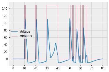
The corresponding plot of n, m, and h is provided to help you debug:
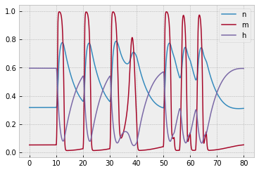
Also, here is a file containing the actual simulation values for t,V,n,m,h:
Lastly, here is a code template:
###############################
### constants

V_0 = ...
n_0 = ...
m_0 = ...
h_0 = ...

C = 1.0
V_Na = 115
...

###############################
### main variables: V, n, m, h

def dV_dt(t,x):
    ...

def dn_dt(t,x):
    V = x['V']
    n = x['n']
    return alpha_n(t,x) * (1-n) - beta_n(t,x) * n

def dm_dt(t,x):
    ...

def dh_dt(t,x):
    ...

###############################
### intermediate variables: alphas, betas, stimulus (s), currents (I's), ...

def alpha_n(t,x):
    ...

def beta_n(t,x):
    ...

...

################################
### input into EulerEstimator

derivatives = {
    'V': dV_dt,
    'n': dn_dt,
    ...
    initial_point = ...
}
Blog Post Preferences
We're going to write some blog posts about things we've done. Check out the posts that the 11th graders wrote last semester: https://www.eurisko.us/blog/
Take a look at this spreadsheet and rank your top 3 posts in order of preference (with 1 being the most preferable). We'll try to match up everyone with a topic they're most interested in.
We're doing this because we need to build up some luck surface area. It's great that we're doing so much cool stuff, but part of the process of opening doors is telling people what you're doing. Writing posts is a way to do that. And, like your Github repositories, blog posts will also help contribute to developing your portfolio so that you have evidence of what you're doing.
Problem 57-2
C++
At the beginning of the year, we wrote a Python function called simple_sort that sorts a list by repeatedly finding the smallest element and appending it to a new list.
Now, you will sort a list in C++ using a similar technique. However, because working with arrays in C++ is a bit trickier, we will modify the implementation so that it only involves the use of a single array. The way we do this is by swapping:
- Find the smallest element in the array
- Swap it with the first element of the array
- Find the next-smallest element in the array
- Swap it with the second element of the array
- ...
For example:
array: [30, 50, 20, 10, 40]
indices to consider: 0, 1, 2, 3, 4
elements to consider: 30, 50, 20, 10, 40
smallest element: 10
swap with first element: [10, 50, 20, 30, 40]

---

array: [10, 50, 20, 30, 40]
indices to consider: 1, 2, 3, 4
elements to consider: 50, 20, 30, 40
smallest element: 20
swap with second element: [10, 20, 50, 30, 40]

---

array: [10, 20, 50, 30, 40]
indices to consider: 2, 3, 4
elements to consider: 50, 30, 40
smallest element: 30
swap with second element: [10, 20, 30, 50, 40]

...

final array: [10, 20, 30, 40, 50]
Write your code in the template below.
# include <iostream>
# inlude <cassert>

int main()
{
    int array[5]{ 30, 50, 20, 10, 40 };

    // your code here

    std::cout << 'Testing...\n';

    assert(array[0]==10);
    assert(array[1]==20);
    assert(array[2]==30);
    assert(array[3]==40);
    assert(array[4]==50);

    std::cout << 'Succeeded';

    return 0;
}
Shell
Complete these Shell coding challenges and submit screenshots. Each screenshot should include your username, the problem title, and the "Status: Accepted" indicator.
Resources:
https://www.thegeekstuff.com/2009/03/15-practical-unix-grep-command-examples/
Problems:
https://www.hackerrank.com/challenges/text-processing-in-linux-the-grep-command-1/problem
https://www.hackerrank.com/challenges/text-processing-in-linux-the-grep-command-2/problem
https://www.hackerrank.com/challenges/text-processing-in-linux-the-grep-command-3/problem
SQL
Complete these SQL coding challenges and submit screenshots. For SQL, each screenshot should include the problem number, the successful smiley face, and your query.
https://sqlzoo.net/wiki/More_JOIN_operations (queries 13, 14, 15)
Problem 57-3
Commit + Review
Commit your code to Github.
Make 1 GitHub issue on your assigned classmate's repository (but NOT
assignment-problems). See eurisko.us/resources/#code-reviews to determine your assigned classmate.Resolve 1 GitHub issue on one of your own repositories.
Submission Template
For your submission, copy and paste your links into the following template:
Repl.it link to Hodgkin-Huxley neuron simulation (make sure it generates the graph): ____
Repl.it link to C++ code: _____
Link to Shell/SQL screenshots (Overleaf or Google Doc): _____

Commit link for simulation repo: _____
Commit link for assignment-problems repo: _____

Created issue: _____
Resolved issue: _____
Problem 56-1
Polynomial Regression
a. The following dataset takes the form $$y = a + bx + cx^2 + dx^3$$ for some constants $a,b,c,d.$ Use linear regression to determine the best-fit values of $a,b,c,d.$ Put your code in the analysis folder and post the values you found on #results once you've got them.
[(0.0, 4.0),
 (0.2, 8.9),
 (0.4, 17.2),
 (0.6, 28.3),
 (0.8, 41.6),
 (1.0, 56.5),
 (1.2, 72.4),
 (1.4, 88.7),
 (1.6, 104.8),
 (1.8, 120.1),
 (2.0, 134.0),
 (2.2, 145.9),
 (2.4, 155.2),
 (2.6, 161.3),
 (2.8, 163.6),
 (3.0, 161.5),
 (3.2, 154.4),
 (3.4, 141.7),
 (3.6, 122.8),
 (3.8, 97.1),
 (4.0, 64.0),
 (4.2, 22.9),
 (4.4, -26.8),
 (4.6, -85.7),
 (4.8, -154.4)]
Tip: To do this, you will need to create a dataset with 3 independent variables ($x, x^2, x^3$) and 1 dependent variable $y.$
To clarify -- the original dataframe looks like this:
>>> df.to_array()
  'x', 'y'
[[0.0, 4.0],
 [0.2, 8.9],
 [0.4, 17.2],
 ...
]
You'll need to transform this dataframe into the following:
>>> df.to_array()
  'x',  'x^2',  'x^3', 'y'
[[0.0, 0.0**2, 0.0**3, 4.0],
 [0.2, 0.2**2, 0.2**3, 8.9],
 [0.4, 0.4**2, 0.4**3, 17.2],
 ...
]
And then you'll fit y as a function of x, x^2, and x^3.
Note: This is a 10-minute problem. If it's taking you longer than that, please post on Slack to get help.
Directed Graph
b. In graph/src/directed_graph.py, create a class DirectedGraph that implements a directed graph.
In a directed graph, nodes have parents and children instead of just "neighbors". For example, a Tree is a special case of an DirectedGraph.
To compute distances and shortest paths in a directed graph, you will use the same approach that you did in the plain old Graph, but instead of considering a node's neighbors each time, you will consider its children.
>>> edges = [(0,1),(1,2),(3,1),(4,3),(1,4),(4,5),(3,6)]
Note: the edges are in the form (parent,child)

>>> directed_graph = DirectedGraph(edges)

at this point, the directed graph looks like this:
0-->1-->2
    ^ \
    |  v
6<--3<--4-->5

>>> [[child.index for child in node.children] for node in directed_graph.nodes]
[[1], [2,4], [], [1,6], [3,5], [], []]

>>> [[parent.index for parent in node.parents] for node in directed_graph.nodes]
[[], [0,3], [1], [4], [1], [4], [3]]

>>> [node.index for node in directed_graph.nodes_breadth_first(4)]
should give a breadth-first ordering, e.g. [4, 3, 5, 6, 1, 2]

>>> [node.index for node in directed_graph.nodes_depth_first(4)]
returns a depth-first ordering, e.g. [4, 3, 6, 1, 2, 5]

>>> directed_graph.calc_distance(0,3)
3
>>> directed_graph.calc_distance(3,5)
3
>>> directed_graph.calc_distance(0,5)
3
>>> directed_graph.calc_distance(4,1)
2
>>> directed_graph.calc_distance(2,4)
False

>>> directed_graph.calc_shortest_path(0,3)
[0, 1, 4, 3]
>>> directed_graph.calc_shortest_path(3,5)
[3, 1, 4, 5]
>>> directed_graph.calc_shortest_path(0,5)
[0, 1, 4, 5]
>>> directed_graph.calc_shortest_path(4,1)
[4, 3, 1]
>>> directed_graph.calc_shortest_path(2,4)
False
Problem 56-2
Haskell
First, observe the following Haskell code which computes the sum of all the squares under 1000:
>>> sum (takeWhile (<1000) (map (^2) [1..]))
10416
(If you don't see why this works, then run each part of the expression: first map (^2) [1..], and then takeWhile (<1000) (map (^2) [1..]), and then the full expression sum (takeWhile (<1000) (map (^2) [1..])).)
Now, recall the Collatz conjecture (if you don't remember it, ctrl+F "collatz conjecture" to jump to the problem where we covered it).
The following Haskell code can be used to recursively generate the sequence or "chain" of Collatz numbers, starting with an initial number n.
chain :: (Integral a) => a -> [a]
chain 1 = [1]
chain n
    | even n =  n:chain (n `div` 2)
    | odd n  =  n:chain (n*3 + 1)
Here are the chains for several initial numbers:
>>> chain 10
[10,5,16,8,4,2,1]
>>> chain 1
[1]
>>> chain 30
[30,15,46,23,70,35,106,53,160,80,40,20,10,5,16,8,4,2,1]
Your problem: Write a Haskell function firstNumberWithChainLengthGreaterThan n that finds the first number whose chain length is at least n.
Check: firstNumberWithChainLengthGreaterThan 15 should return 7.
To see why this check works, observe the first few chains shown below:
1: [1] (length 1)
2: [2,1] (length 2)
3: [3,10,5,16,8,4,2,1] (length 8)
4: [4,2,1] (length 3)
5: [5,16,8,4,2,1] (length 6)
6: [6,3,10,5,16,8,4,2,1] (length 9)
7: [7,22,11,34,17,52,26,13,40,20,10,5,16,8,4,2,1] (length 17)
7 is the first number whose chain is at least 15 numbers long.
Shell
Complete these Shell coding challenges and submit screenshots. Each screenshot should include your username, the problem title, and the "Status: Accepted" indicator.
Helpful resources:
https://www.geeksforgeeks.org/awk-command-unixlinux-examples/
https://www.thegeekstuff.com/2010/02/awk-conditional-statements/
Problems:
SQL
Complete these SQL coding challenges and submit screenshots. For SQL, each screenshot should include the problem number, the successful smiley face, and your query.
https://sqlzoo.net/wiki/More_JOIN_operations (queries 9, 10, 11, 12)
Problem 56-3
Commit + Review
Commit your code to Github.
Make 1 GitHub issue on your assigned classmate's repository (but NOT
assignment-problems). See eurisko.us/resources/#code-reviews to determine your assigned classmate.Resolve 1 GitHub issue on one of your own repositories.
Submission Template
For your submission, copy and paste your links into the following template:
Repl.it link to polynomial regression code: ___
Repl.it link to directed graph tests: ___

Repl.it link to Haskell code: _____
Link to Shell/SQL screenshots (Overleaf or Google Doc): _____

Commit link for assignment-problems repo: _____
Commit link for graph repo: _____
Commit link for machine-learning repo: _____

Created issue: _____
Resolved issue: _____
Problem 56-4
There will be a 45-minute quiz that you can take any time on Thursday. (We don't have school Friday.)
The quiz will cover C++ and Haskell.
For C++, you will need to be comfortable working with arrays.
For Haskell, you'll need to be comfortable working with list comprehensions and compositions of functions.
You will need to write C++ and Haskell functions to calculate some values. It will be somewhat similar to the meta-Fibonacci sum problem, except the computation will be different (and simpler).
Problem 55-1
Location: assignment-problems/magic_square.py
In this problem, you will solve for all arrangements of digits $1,2,\ldots, 9$ in a $3 \times 3$ "magic square" where all the rows, columns, and diagonals add up to $15$ and no digits are repeated.
a.
First, create a function is_valid(arr) that checks if a possibly-incomplete array is a valid magic square "so far". In order to be valid, all the rows, columns, and diagonals in an array that have been completely filled in must sum to $15.$
>>> arr1 = [[1,2,None],
           [None,3,None],
           [None,None,None]]
>>> is_valid(arr1)
True    (because no rows, columns, or diagonals are completely filled in)

>>> arr2 = [[1,2,None],
           [None,3,None],
           [None,None,4]]
>>> is_valid(arr2)
False   (because a diagonal is filled in and it doesn't sum to 15)

>>> arr3 = [[1,2,None],
           [None,3,None],
           [5,6,4]]
>>> is_valid(arr3)
False   (because a diagonal is filled in and it doesn't sum to 15)
        (it doesn't matter that the bottom row does sum to 15)

>>> arr4 = [[None,None,None],
           [None,3,None],
           [5,6,4]]
>>> is_valid(arr4)
True   (because there is one row that's filled in and it sums to 15)
b.
Now, write a script to start filling in numbers of the array -- but whenever you reach a configuration that can no longer become a valid magic square, you should not explore that configuration any further. Once you reach a valid magic square, print it out.
- Tip: An ugly but straightforward way to solve this is to use 9 nested
forloops, along withcontinuestatements where appropriate. (Acontinuestatement allows you to immediately continue to the next item in aforloop, without executing any of the code below thecontinuestatement.)
Some of the first steps are shown below to give a concrete demonstration of the procedure:
Filling...

[[_,_,_],
 [_,_,_],
 [_,_,_]]

[[1,_,_],
 [_,_,_],
 [_,_,_]]

[[1,2,_],
 [_,_,_],
 [_,_,_]]

[[1,2,3],
 [_,_,_],
 [_,_,_]]

^ is no longer a valid magic square

[[1,2,4],
 [_,_,_],
 [_,_,_]]

^ is no longer a valid magic square

[[1,2,5],
 [_,_,_],
 [_,_,_]]

^ is no longer a valid magic square

...

[[1,2,9],
 [_,_,_],
 [_,_,_]]

^ is no longer a valid magic square

[[1,3,2],
 [_,_,_],
 [_,_,_]]

^ is no longer a valid magic square

[[1,3,4],
 [_,_,_],
 [_,_,_]]

^ is no longer a valid magic square

[[1,3,5],
 [_,_,_],
 [_,_,_]]

^ is no longer a valid magic square

...

[[1,3,9],
 [_,_,_],
 [_,_,_]]

^ is no longer a valid magic square

[[1,4,2],
 [_,_,_],
 [_,_,_]]

^ is no longer a valid magic square

...

[[1,5,9],
 [_,_,_],
 [_,_,_]]

[[1,5,9],
 [2,_,_],
 [_,_,_]]

[[1,5,9],
 [2,3,_],
 [_,_,_]]

[[1,5,9],
 [2,3,4],
 [_,_,_]]

^ is no longer a valid magic square

[[1,5,9],
 [2,3,5],
 [_,_,_]]

^ is no longer a valid magic square

...
Here is a rough outline of the structure:
arr = (initialize it with Nones)
for num1 in range(1,10):
    clear out the array and put num1 in it
    if not is_valid(arr):
        continue
    for num2 in range(1,10): # modify this range so that it doesn't include num1
        clear out the array and put num1, num2 in it
        if not is_valid(arr):
            continue
        for num3 in range(1,10): # modify this range so that it doesn't include num1 nor num2
            clear out the array and put num1, num2, num3 in it
            if not is_valid(arr):
                continue
            ... and so on
Problem 55-2
C++
Implement the metaFibonacciSum function in C++:
# include <iostream>
# include <cassert>

int metaFibonacciSum(int n)
{
    // return the result immediately if n<2

    // otherwise, construct a an array called "terms"
    // that contains the Fibonacci terms at indices
    // 0, 1, ..., n

    // construct an array called "extendedTerms" that
    // contains the Fibonacci terms at indices
    // 0, 1, ..., a_n (where a_n is the nth Fibonacci term)

    // when you fill up this array, many of the terms can
    // simply copied from the existing "terms" array. But
    // if you need additional terms, you'll have to compute
    // them the usual way (by adding the previous 2 terms)

    // then, create an array called "partialSums" that
    // contains the partial sums S_0, S_1, ..., S_{a_n}

    // finally, add up the desired partial sums,
    // S_{a_0} + S_{a_1} + ... + S_{a_n},
    // and return this result

}

int main()
{
    std::cout << "Testing...\n";

    assert(metaFibonacciSum(6)==74);

    std::cout << "Success!";

    return 0;
}
Shell
Complete these Shell coding challenges and submit screenshots. Each screenshot should include your username, the problem title, and the "Status: Accepted" indicator.
Helpful resource: https://www.geeksforgeeks.org/awk-command-unixlinux-examples/
SQL
Complete these SQL coding challenges and submit screenshots. For SQL, each screenshot should include the problem number, the successful smiley face, and your query.
https://sqlzoo.net/wiki/More_JOIN_operations (queries 5, 6, 7, 8)
Problem 55-3
Review; 10% of assignment grade; 15 minutes estimate
Commit your code to Github.
Make 1 GitHub issue on your assigned classmate's repository (but NOT
assignment-problems). See eurisko.us/resources/#code-reviews to determine your assigned classmate.Resolve 1 GitHub issue on one of your own repositories.
SUBMISSION TEMPLATE
For your submission, copy and paste your links into the following template:
Repl.it link to magic square solver: ___

Repl.it link to C++ code: _____
Link to Shell/SQL screenshots (Overleaf or Google Doc): _____

Commit link for assignment-problems repo: _____

Created issue: _____
Resolved issue: _____
Problem 54-1
Primary problems; 60% of assignment grade; 60 minutes estimate
In your Graph class, create a method graph.set_breadth_first_distance_and_previous(starting_node_index) that does a breadth-first traversal and sets the attributes node.distance and node.previous during the traversal.
Whenever you're at a current_node, and you check the neighbors, make the following updates
set
neighbor.previousas thecurrent_nodeset
neighbor.distance = current_node.distance + 1
Then, create the following methods:
graph.calc_distance(starting_node_index, ending_node_index)- computes the distance between the starting node and the ending node. All you have to do is rungraph.set_breadth_first_distance_and_previous(starting_node_index)and then return thedistanceof theending_node.graph.calc_shortest_path(starting_node_index, ending_node_index)- computes the sequence of node indices on the shortest path between the starting node and the ending node. All you have to do isrun
graph.set_breadth_first_distance_and_previous(starting_node_index)start at the terminal node and repeatedly go to the previous node until you get to the initial node
keep track of all the nodes you visit (this is the shortest path in reverse)
return the path in order from the initial node index to the terminal node index (you'll have to reverse the reversed path)
Here are some tests:
>>> edges = [(0,1),(1,2),(1,3),(3,4),(1,4),(4,5)]
>>> graph = Graph(edges)

at this point, the graph looks like this:
0 -- 1 -- 2
     | \
     3--4 -- 5

>>> graph.calc_distance(0,4)
2
>>> graph.calc_distance(5,2)
3
>>> graph.calc_distance(0,5)
3
>>> graph.calc_distance(4,1)
1
>>> graph.calc_distance(3,3)
0

>>> graph.calc_shortest_path(0,4)
[0, 1, 4]
>>> graph.calc_shortest_path(5,2)
[5, 4, 1, 2]
>>> graph.calc_shortest_path(0,5)
[0, 1, 4, 5]
>>> graph.calc_shortest_path(4,1)
[4, 1]
>>> graph.calc_shortest_path(3,3)
[3]
Problem 54-2
Supplemental problems; 30% of assignment grade; 60 minutes estimate
Location: assignment-problems
Haskell
Let $a_k$ be the $k$th Fibonacci number and let $S_k$ be the sum of the first $k$ Fibonacci numbers. Write a function metaFibonacciSum that takes an input $n$ and computes the sum
For example, if we wanted to compute the result for n=6, then we'd need to
compute the first $6$ Fibonacci numbers: $$ a_0=0, a_1=1, a_2=1, a_3=2, a_4=3, a_5=5, a_6=8 $$
compute the first $8$ Fibonacci sums: $$ \begin{align*} S_0 &= 0 \\ S_1 &= 0 + 1 = 1 \\ S_2 &= 0 + 1 + 1 = 2 \\ S_3 &= 0 + 1 + 1 + 2 = 4 \\ S_4 &= 0 + 1 + 1 + 2 + 3 = 7 \\ S_5 &= 0 + 1 + 1 + 2 + 3 + 5 = 12 \\ S_6 &= 0 + 1 + 1 + 2 + 3 + 5 + 8 = 20 \\ S_7 &= 0 + 1 + 1 + 2 + 3 + 5 + 8 + 13 = 33 \\ S_8 &= 0 + 1 + 1 + 2 + 3 + 5 + 8 + 13 + 21 = 54 \\ \end{align*} $$
Add up the desired sums:
$$ \begin{align*} \sum\limits_{k=0}^6 S_{a_k} &= S_{a_0} + S_{a_1} + S_{a_2} + S_{a_3} + S_{a_4} + S_{a_5} + S_{a_6} \\ &= S_{0} + S_{1} + S_{1} + S_{2} + S_{3} + S_{5} + S_{8} \\ &= 0 + 1 + 1 + 2 + 4 + 12 + 54 \\ &= 74 \end{align*} $$Here's a template:
-- first, define a recursive function "fib"
-- to compute the nth Fibonacci number

-- once you've defined "fib", proceed to the
-- steps below
firstKEntriesOfSequence k = -- your code here; should return the list [a_0, a_1, ..., a_k]
kthPartialSum k = -- your code here; returns a single number
termsToAddInMetaSum n = -- your code here; should return the list [S_{a_0}, S_{a_1}, ..., S_{a_k}]
metaSum n = -- your code here; returns a single number

main = print (metaSum 6) -- should come out to 74
Shell
Complete these Shell coding challenges and submit screenshots. Each screenshot should include your username, the problem title, and the "Status: Accepted" indicator.
Helpful resource: https://www.theunixschool.com/2012/07/10-examples-of-paste-command-usage-in.html
https://www.hackerrank.com/challenges/paste-1/problem
https://www.hackerrank.com/challenges/paste-2/problem
SQL
Complete these SQL coding challenges and submit screenshots. For SQL, each screenshot should include the problem number, the successful smiley face, and your query.
https://sqlzoo.net/wiki/More_JOIN_operations (queries 1, 2, 3, 4)
Problem 54-3
Review; 10% of assignment grade; 15 minutes estimate
Commit your code to Github.
Make 1 GitHub issue on your assigned classmate's repository (but NOT
assignment-problems). See eurisko.us/resources/#code-reviews to determine your assigned classmate.Resolve 1 GitHub issue on one of your own repositories.
SUBMISSION TEMPLATE
For your submission, copy and paste your links into the following template:
Repl.it link to graph/tests/test_graph.py: ___

Repl.it link to Haskell code: _____
Link to Shell/SQL screenshots (Overleaf or Google Doc): _____

Commit link for space-empires repo: _____
Commit link for assignment-problems repo: _____

Created issue: _____
Resolved issue: _____
Problem 53-1
Primary problems; 60% of assignment grade; 60 minutes estimate
In your LinearRegressor and LogisticRegressor, in your predict method, update your observation as follows:
If there are any non-interaction terms (i.e. doesn't contain a '*' symbol) as dataframe columns, that do not appear in your observation, then set their observation values to $0.$
If there are any interaction terms that appear as dataframe columns, but do not appear in your observation, then generate them.
Then, you should be able to run the following tests (taken from Problem 52-1)
# test 8 slices of beef + mayo
>>> observation = {'beef': 8, 'mayo': 1}
>>> linear_regressor.predict(observation)
11.34
>>> logistic_regressor.predict(observation)
9.72

Note: under the hood, the observation should be transformed like this:

initial input:
    {'beef': 8, 'mayo': 1}

fill in 0's for any missing non-interaction variables:
    {'beef': 8, 'pb': 0, 'mayo': 1, 'jelly': 0}

fill in missing interaction terms that appear in the dataset:
    {'beef': 8, 'pb': 0, 'mayo': 1, 'jelly': 0,
    'beef * pb': 0, 'beef * mayo': 8, 'beef * jelly': 0,
    'pb * mayo': 0, 'pb * jelly': 0,
    'mayo * jelly': 0}

# test 4 tbsp of pb + 8 slices of beef + mayo
>>> observation = {'beef': 8, 'pb': 4, 'mayo': 1}
>>> linear_regressor.predict(observation)
3.62
>>> logistic_regressor.predict(observation)
0.77

# test 8 slices of beef + mayo + jelly
>>> observation = {'beef': 8, 'mayo': 1, 'jelly': 1}
>>> linear_regressor.predict(observation)
2.79
>>> logistic_regressor.predict(observation)
0.79
b. Submit quiz corrections for any problems you missed. We went over the quiz in the first part of the class recording: https://vimeo.com/507190028
(Note: if you did not miss any problems, then you don't have to submit anything)
Problem 53-2
Supplemental problems; 30% of assignment grade; 60 minutes estimate
Location: assignment-problems
a. Skim the following section of http://learnyouahaskell.com/higher-order-functions.
Function composition
Consider the function $$ f(x,y) = \max \left( x, -\tan(\cos(y)) \right) $$
This function can be implemented as
>>> f x y = negate (max (x tan (cos y)))or, we can implement it using function composition notation as follows:
>>> f x = negate . max x . tan . cosNote that although max is a function of two variables, max x is a function of one variable (since one of the inputs is already supplied). So, we can chain it together with other single-variable functions.
Previously, you wrote a function tail' in Tail.hs that finds the last n elements of a list by reversing the list, finding the head n elements of the reversed list, and then reversing the result.
Rewrite the function tail' using composition notation, so that it's cleaner. Run Tail.hs again to make sure it still gives the same output as before.
b. Write a function isPrime that determines whether a nonnegative integer x is prime. You can use the same approach that you did with one of our beginning Python problems: loop through numbers between 2 and x-1 and see if you can find any factors.
Note that neither 0 nor 1 are prime.
Here is a template for your file isPrime.cpp:
#include <iostream>
#include <cassert>

bool isPrime(int x)
{
    // your code here
}

int main()
{
    assert(!isPrime(0));
    assert(!isPrime(1));
    assert(isPrime(2));
    assert(isPrime(3));
    assert(!isPrime(4));
    assert(isPrime(5));
    assert(isPrime(7));
    assert(!isPrime(9));
    assert(isPrime(11));
    assert(isPrime(13));
    assert(!isPrime(15));
    assert(!isPrime(16));
    assert(isPrime(17));
    assert(isPrime(19));
    assert(isPrime(97));
    assert(!isPrime(99));
    assert(!isPrime(99));
    assert(isPrime(13417));

    std::cout << "Success!";

    return 0;
}
Your program should work like this
>>> g++ isPrime.cpp -o isPrime
>>> ./isPrime
Success!
c. Complete these Shell coding challenges and submit screenshots. Each screenshot should include your username, the problem title, and the "Status: Accepted" indicator.
Here's a reference to the sort command: https://www.thegeekstuff.com/2013/04/sort-files/
Note that the "tab" character must be specified as $'\t'.
These problems are super quick, so we'll do several.
https://www.hackerrank.com/challenges/text-processing-sort-5/tutorial
https://www.hackerrank.com/challenges/text-processing-sort-6/tutorial
https://www.hackerrank.com/challenges/text-processing-sort-7/tutorial
d. Complete these SQL coding challenges and submit screenshots. For SQL, each screenshot should include the problem number, the successful smiley face, and your query.
https://sqlzoo.net/wiki/The_JOIN_operation (queries 12, 13)
Problem 53-3
Review; 10% of assignment grade; 15 minutes estimate
Commit your code to Github.
Make 1 GitHub issue on your assigned classmate's repository (but NOT
assignment-problems). See eurisko.us/resources/#code-reviews to determine your assigned classmate.Resolve 1 GitHub issue on one of your own repositories.
SUBMISSION TEMPLATE
For your submission, copy and paste your links into the following template:
Repl.it link to machine-learning/tests/test_logistic_regressor.py: _____
Repl.it link to machine-learning/tests/test_linear_regressor.py: _____
Overleaf link to quiz corrections: _____

Repl.it link to Haskell code: _____
Repl.it link to C++ code: _____
Link to Shell/SQL screenshots (Overleaf or Google Doc): _____

Commit link for machine-learning repo: _____
Commit link for assignment-problems repo: _____

Created issue: _____
Resolved issue: _____
Problem 52-1
Primary problems; 60% of assignment grade; 60 minutes estimate
a. Consider the sandwich prediction task again.
>>> df = DataFrame.from_array(
    [[0, 0, [],               1],
    [0, 0, ['mayo'],          1],
    [0, 0, ['jelly'],         4],
    [0, 0, ['mayo', 'jelly'], 0],
    [5, 0, [],                4],
    [5, 0, ['mayo'],          8],
    [5, 0, ['jelly'],         1],
    [5, 0, ['mayo', 'jelly'], 0],
    [0, 5, [],                5],
    [0, 5, ['mayo'],          0],
    [0, 5, ['jelly'],         9],
    [0, 5, ['mayo', 'jelly'], 0],
    [5, 5, [],                0],
    [5, 5, ['mayo'],          0],
    [5, 5, ['jelly'],         0],
    [5, 5, ['mayo', 'jelly'], 0]],
    columns = ['beef', 'pb', 'condiments', 'rating']
)
(i) Fit a linear regression model containing all interaction terms. Put the model it in an Overleaf doc.
rating = beta_0
         + beta_1 ( slices beef ) + beta_2 ( tbsp pb ) + beta_3 ( mayo ) + beta_4 ( jelly )
         + beta_5 ( slices beef ) ( tbsp pb ) + beta_6 ( slices beef ) ( mayo ) + beta_7 ( slices beef ) ( jelly )
         + beta_8 ( tbsp pb ) ( mayo ) + beta_9 ( tbsp pb ) ( jelly )
         + beta_10 ( mayo ) ( jelly )
(ii) Fit a logistic regression model containing all interaction terms. Whever there is a rating of 0, replace it with 0.1. Put the model in an Overleaf doc.
rating = 10/(1 + exp(
                    beta_0
                    + beta_1 ( slices beef ) + beta_2 ( tbsp pb ) + beta_3 ( mayo ) + beta_4 ( jelly )
                    + beta_5 ( slices beef ) ( tbsp pb ) + beta_6 ( slices beef ) ( mayo ) + beta_7 ( slices beef ) ( jelly )
                    + beta_8 ( tbsp pb ) ( mayo ) + beta_9 ( tbsp pb ) ( jelly )
                    + beta_10 ( mayo ) ( jelly ) ))
(iii) Use your models to predict the following ratings. Post your predictions on #results once you've got them.
8 slices of beef + mayo
    linear regression rating prediction: ___
    logistic regression rating prediction: ___

4 tbsp of pb + jelly
    linear regression rating prediction: ___
    logistic regression rating prediction: ___

4 tbsp of pb + mayo
    linear regression rating prediction: ___
    logistic regression rating prediction: ___

4 tbsp of pb + 8 slices of beef + mayo
    linear regression rating prediction: ___
    logistic regression rating prediction: ___

8 slices of beef + mayo + jelly
    linear regression rating prediction: ___
    logistic regression rating prediction: ___
b. Create a Graph class in your graph repository. This will represent an undirected graph, so instead of parents and children, nodes will merely have neighbors. An edge (a,b) means a is a neighbor of b and b is a neighbor of a. So the order of a and b does not matter.
Implement a method
get_nodes_breadth_firstthat returns the nodes in breadth-first order.Implement a method
get_nodes_depth_firstthat returns the nodes in depth-first order.
These methods will be almost exactly the same as in your Tree class, except it should only consider neighbors that are unvisited and not in the queue. Also, we will need to pass in the index of the starting node.
Note: Originally, I intended for us to write a calc_distance method that works similarly to breadth-first search, but on second thought, we should start by implementing breadth-first and depth-first search in our Graph class since it's slightly different than what we implemented in the Tree class. We'll do calc_distance on the next assignment.
>>> edges = [(0,1),(1,2),(1,3),(3,4),(1,4),(4,5)]
>>> graph = Graph(edges)

the graph looks like this:
0 -- 1 -- 2
     | \
     3--4 -- 5

>>> bf = graph.get_nodes_breadth_first(2)
>>> [node.index for node in bf]
[2, 1, 0, 3, 4, 5]

note: other breadth-first orders are permissible,
e.g. [2, 1, 4, 3, 0, 5]

here's what's happening under the hood:

    queue = [2], visited = []

    current_node: 2
    unvisited neighbors not in queue: 1

    queue = [1], visited = [2]

    current_node: 1
    unvisited neighbors not in queue: 0, 3, 4

    queue = [0, 3, 4], visited = [2, 1]

    current_node: 0
    unvisited neighbors not in queue: (none)

    queue = [3, 4], visited = [2, 1, 0]

    current_node: 3
    unvisited neighbors not in queue: (none)

    queue = [4], visited = [2, 1, 0, 3]

    current_node: 4
    unvisited neighbors not in queue: 5

    queue = [5], visited = [2, 1, 0, 3, 4]

    current_node: 5
    unvisited neighbors not in queue: (none)

    queue = [], visited = [2, 1, 0, 3, 4, 5]

    queue is empty, so we stop

>>> df = graph.get_nodes_depth_first(2)
>>> [node.index for node in df]
[2, 1, 3, 4, 5, 0]

note: other depth-first orders are permissible,
e.g. [2, 1, 4, 5, 3, 0]
Problem 52-2
Supplemental problems; 30% of assignment grade; 60 minutes estimate
Location: assignment-problems
a. Skim the following section of http://learnyouahaskell.com/higher-order-functions.
Maps and filters
Pay attention to the following examples:
>>> map (+3) [1,5,3,1,6]
[4,8,6,4,9]
>>> filter (>3) [1,5,3,2,1,6,4,3,2,1]
[5,6,4]
Create a Haskell file SquareSingleDigitNumbers.hs and write a function squareSingleDigitNumbers that takes a list returns the squares of the values that are less than 10.
To check your function, print squareSingleDigitNumbers [2, 7, 15, 11, 5]. You should get a result of [4, 49, 25].
This is a one-liner. If you get stuck for more than 10 minutes, ask for help on Slack.
b. Write a C++ program to calculate the height of a ball that falls from a tower.
- Create a file
constants.hto hold your gravity constant:
#ifndef CONSTANTS_H
#define CONSTANTS_H

namespace myConstants
{
    const double gravity(9.8); // in meters/second squared
}
#endif- Create a file
simulateFall.cpp
#include <iostream>
#include "constants.h"

double calculateDistanceFallen(int seconds)
{
    // approximate distance fallen after a particular number of seconds
    double distanceFallen = myConstants::gravity * seconds * seconds / 2;

    return distanceFallen;
}

void printStatus(int time, double height)
{
    std::cout << "At " << time
    << " seconds, the ball is at height "
    << height << " meters\n";
}

int main()
{
    using namespace std;
    cout << "Enter the initial height of the tower in meters: ";
    double initialHeight;
    cin >> initialHeight;

    // your code here
    // use calculateDistanceFallen to find the height now

    // use calculateDistanceFallen and printStatus
    // to generate the desired output
    // if the height now goes negative, then the status
    // should say that the height is 0 and the program
    // should stop (since the ball stops falling at height 0)

    return 0;
}
Your program should work like this
>>> g++ simulateFall.cpp -o simulateFall
>>> ./simulateFall
Enter the initial height of the tower in meters: 100
At 0 seconds, the ball is at height 100 meters
At 1 seconds, the ball is at height 95.1 meters
At 2 seconds, the ball is at height 80.4 meters
At 3 seconds, the ball is at height 55.9 meters
At 4 seconds, the ball is at height 21.6 meters
At 5 seconds, the ball is at height 0 meters
c. Complete these Shell coding challenges and submit screenshots. Each screenshot should include your username, the problem title, and the "Status: Accepted" indicator.
Here's a reference to the sort command: https://www.thegeekstuff.com/2013/04/sort-files/
These problems are super quick, so we'll do several.
https://www.hackerrank.com/challenges/text-processing-sort-1/tutorial
https://www.hackerrank.com/challenges/text-processing-sort-2/tutorial
https://www.hackerrank.com/challenges/text-processing-sort-3/tutorial
https://www.hackerrank.com/challenges/text-processing-sort-4/tutorial
d. Complete these SQL coding challenges and submit screenshots. For SQL, each screenshot should include the problem number, the successful smiley face, and your query.
https://sqlzoo.net/wiki/The_JOIN_operation (queries 10, 11)
Problem 52-3
Review; 10% of assignment grade; 15 minutes estimate
Now, everyone should have a handful of issues on their repositories. So we'll go back to making 1 issue and resolving 1 issue.
Make 1 GitHub issues on your assigned classmate's repository (but NOT
assignment-problems). See eurisko.us/resources/#code-reviews to determine your assigned classmate.Resolve 1 GitHub issue on one of your own repositories.
SUBMISSION TEMPLATE
For your submission, copy and paste your links into the following template:
Link to Overleaf doc containing your model: _____

Link to file in machine-learning/analysis where you fit
your regressors with dummy variables and interaction terms: ____

Link to graph/tests/test_graph.py: _____

Repl.it link to Haskell code: _____
Repl.it link to C++ code: _____
Link to Shell/SQL screenshots (Overleaf or Google Doc): _____

Commit link for machine-learning repo: _____
Commit link for graph repo: _____
Commit link for assignment-problems repo: _____

Created issue: _____
Resolved issue: _____
Problem 51-1
Primary problems; 60% of assignment grade; 60 minutes estimate
a. In your dataframe, write a method create_dummy_variables().
>>> df = DataFrame.from_array(
    [[0, 0, [],               1],
    [0, 0, ['mayo'],          1],
    [0, 0, ['jelly'],         4],
    [0, 0, ['mayo', 'jelly'], 0],
    [5, 0, [],                4],
    [5, 0, ['mayo'],          8],
    [5, 0, ['jelly'],         1],
    [5, 0, ['mayo', 'jelly'], 0],
    [0, 5, [],                5],
    [0, 5, ['mayo'],          0],
    [0, 5, ['jelly'],         9],
    [0, 5, ['mayo', 'jelly'], 0],
    [5, 5, [],                0],
    [5, 5, ['mayo'],          0],
    [5, 5, ['jelly'],         0],
    [5, 5, ['mayo', 'jelly'], 0]],
    columns = ['beef', 'pb', 'condiments', 'rating']
)

>>> df = df.create_dummy_variables('condiments')

>>> df.columns
['beef', 'pb', 'mayo', 'jelly', 'rating']

>>> df.to_array()
[[0, 0, 0, 0, 1],
[0, 0, 1, 0, 1],
[0, 0, 0, 1, 4],
[0, 0, 1, 1, 0],
[5, 0, 0, 0, 4],
[5, 0, 1, 0, 8],
[5, 0, 0, 1, 1],
[5, 0, 1, 1, 0],
[0, 5, 0, 0, 5],
[0, 5, 1, 0, 0],
[0, 5, 0, 1, 9],
[0, 5, 1, 1, 0],
[5, 5, 0, 0, 0],
[5, 5, 1, 0, 0],
[5, 5, 0, 1, 0],
[5, 5, 1, 1, 0]]
b. Suppose that you wish to model a deer population $D(t)$ and a wolf population $W(t)$ over time $t$ (where time is measured in years).
Initially, there are $100$ deer and $10$ wolves.
In the absence of wolves, the deer population would increase at the instantaneous rate of $60\%$ per year.
In the absence of deer, the wolf population would decrease at the instantaneous rate of $90\%$ per year.
The wolves and deer meet at an instantaneous rate of $0.05$ times per wolf per deer per year, and every time a wolf meets a deer, it kills and eats the deer.
The rate at which the wolf population increases is proportional to the number of deer that are killed, by a factor of $0.4.$ In other words, the wolf population grows by a rate of $0.4$ wolves per deer killed per year.
(i) Set up a system of differential equations to model the situation:
\begin{cases} \dfrac{\text{d}D}{\textrm{d}t} = (\_\_\_) D + (\_\_\_) DW, \quad D(0) = \_\_\_ \\ \dfrac{\text{d}W}{\textrm{d}t} = (\_\_\_) W + (\_\_\_) DW, \quad W(0) = \_\_\_ \\ \end{cases}Check your answer: at $t=0,$ you should have $\dfrac{\text{d}D}{\textrm{d}t} = 10$ and $\dfrac{\text{d}W}{\textrm{d}t} = 11.$
IMPORTANT: Don't spend too long setting up your system. If you've spent over 10 minutes on it, and your system doesn't pass the check, then send a screenshot of your system to me and I'll give you some guidance.
Here's some latex for you to use:
$$\begin{cases}
\dfrac{\text{d}D}{\textrm{d}t} = (\_\_\_) D + (\_\_\_) DW, \quad D(0) = \_\_\_ \\
\dfrac{\text{d}W}{\textrm{d}t} = (\_\_\_) W + (\_\_\_) DW, \quad W(0) = \_\_\_ \\
\end{cases}$$
(ii) (2 points) Plot the system of differential equations for $0 \leq t \leq 100,$ using a step size $\Delta t = 0.001.$ Put this plot in your Overleaf doc and post it on results.
- Check: Your plot should display oscillations, like a sinusoidal curve.
(iii) Explain why the oscillations arise. What does this mean in terms of the wolf and deer populations? Why does this happen?
Problem 51-2
Supplemental problems; 30% of assignment grade; 60 minutes estimate
PART 1
Location: assignment-problems
Skim the following section of http://learnyouahaskell.com/recursion.
A few more recursive functions
Pay attention to the following example. take n myList returns the first n entries of myList.
take' :: (Num i, Ord i) => i -> [a] -> [a]
take' n _
    | n <= 0   = []
take' _ []     = []
take' n (x:xs) = x : take' (n-1) xs
Create a Haskell file Tail.hs and write a function tail' that takes a list and returns the last n values of the list.
Here's the easiest way to do this...
Write a helper function
reverseListthat reverses a list. This will be a recursive function, which you can define using the following template:reverseList :: [a] -> [a] reverseList [] = (your code here -- base case) reverseList (x:xs) = (your code here -- recursive formula)Here,
xis the first element of the input list andxsis the rest of the elements. For the recursive formula, just callreverseListon the rest of the elements and put the first element of the list at the end. You'll need to use the++operation for list concatenation.Once you've written
reverseListand tested to make sure it works as intended, you can implementtail'by reversing the input list, callingtake'on the reversed list, and reversing the result.
To check your function, print tail' 4 [8, 3, -1, 2, -5, 7]. You should get a result of [-1, 2, -5, 7].
If you get stuck anywhere in this problem, don't spend a bunch of time staring at it. Be sure to post on Slack. These Haskell problems can be tricky if you're not taking the right approach from the beginning, but after a bit of guidance, it can become much simpler.
PART 2
Complete these C++/Shell/SQL coding challenges and submit screenshots.
For C++/Shell, each screenshot should include your username, the problem title, and the "Status: Accepted" indicator.
For SQL, each screenshot should include the problem number, the successful smiley face, and your query.
C++
https://www.hackerrank.com/challenges/inheritance-introduction/problem
- Guess what? After this problem, we're done with the useful C++ problems on HackerRank. Next time, we'll start some C++ coding in Repl.it. We'll start by re-implementing a bunch of problems that we did when we were first getting used to Python.
Shell
https://www.hackerrank.com/challenges/text-processing-tr-1/problem
https://www.hackerrank.com/challenges/text-processing-tr-2/problem
https://www.hackerrank.com/challenges/text-processing-tr-3/problem
Helpful templates:
$ echo "Hello" | tr "e" "E"
HEllo
$ echo "Hello how are you" | tr " " '-'
Hello-how-are-you
$ echo "Hello how are you 1234" | tr -d [0-9]
Hello how are you
$ echo "Hello how are you" | tr -d [a-e]
Hllo how r you
More info on
trhere: https://www.thegeekstuff.com/2012/12/linux-tr-command/These problems are all very quick. If you find yourself spending more than a couple minutes on these, be sure to ask for help.
SQL
https://sqlzoo.net/wiki/The_JOIN_operation (queries 7, 8, 9)
Problem 51-3
Review; 10% of assignment grade; 15 minutes estimate
Commit your code to GitHub. When you submit your assignment, include a link to your commit(s). If you don't do this, your assignment will receive a grade of $0$ until you resubmit with links to your commits.
Additionally, do the following:
- Make 2 GitHub issues on your assigned classmate's repository (but NOT
assignment-problems). See eurisko.us/resources/#code-reviews to determine your assigned classmate. When you submit your assignment, include the links to the issues you created.
SUBMISSION TEMPLATE
For your submission, copy and paste your links into the following template:
Repl.it link to dataframe tests including create_dummy_variables: _____
Repl.it link to predator_prey_model.py: _____
Link to Overleaf doc: _____

Repl.it link to Haskell code: _____
Link to C++/Shell/SQL screenshots (Overleaf or Google Doc): _____

Commit link for simulation repo: _____
Commit link for machine-learning repo: _____
Commit link for assignment-problems repo: _____

Issue 1: _____
Issue 2: _____
Problem 50-1
Primary problems; 60% of assignment grade; 60 minutes estimate
Location: Overleaf and simulation/analysis/sir_model.py
One of the simplest ways to model the spread of disease using differential equations is the SIR model. The SIR model assumes three sub-populations: susceptible, infected, and recovered.
The number of susceptible people $(S)$ decreases at a rate proportional to the rate of meeting between susceptible and infected people (because susceptible people have a chance of catching the disease when they come in contact with infected people).
The number of infected people $(I)$ increases at a rate proportional to the rate of meeting between susceptible and infected people (because susceptible people become infected after catching the disease), and decreases at a rate proportional to the number of infected people (as the diseased people recover).
The number of recovered people $(R)$ increases at a rate proportional to the number of infected people (as the diseased people recover).
a. Write a system of differential equations to model the system. Put your system in an Overleaf doc.
$$\begin{cases} \dfrac{\textrm{d}S}{\textrm{d}t} &= \_\_\_, \quad S(0) = \_\_\_ \\ \dfrac{\textrm{d}I}{\textrm{d}t} &= \_\_\_, \quad I(0) = \_\_\_ \\ \dfrac{\textrm{d}R}{\textrm{d}t} &= \_\_\_, \quad R(0) = \_\_\_ \end{cases}$$Make the following assumptions:
There are initially $1000$ susceptible people and $1$ infected person.
The number of meetings between susceptible and infected people each day is proportional to the product of the numbers of susceptible and infected people, by a factor of $0.01 \, .$ The transmission rate of the disease is $3\%.$ (In other words, $3\%$ of meetings result in transmission.)
Each day, $2\%$ of infected people recover.
Check: If you've written the system correctly, then at $t=0,$ you should have
$$ \dfrac{\textrm{d}S}{\textrm{d}t} = -0.3, \quad \dfrac{\textrm{d}I}{\textrm{d}t} = 0.28, \quad \dfrac{\textrm{d}R}{\textrm{d}t} = 0.02 \, . $$IMPORTANT: Don't spend too long setting up your system. If you've spent over 10 minutes on it, and your system doesn't pass the check, then send a screenshot of your system to me and I'll give you some guidance.
b. Plot the system, post your plot on #results, and include the plot in your Overleaf document.
You get to choose your own step size and interval. Choose a step size small enough that the model doesn't blow up, but large enough that the simulation doesn't take long to run.
Choose an interval that displays all the main features of the differential equation, i.e. an interval that shows the behavior of the curves until they start to asymtpote off.
c. Describe the plot in words, explaining what is happening in the plot and why it is happening.
Problem 50-2
Supplemental problems; 30% of assignment grade; 60 minutes estimate
PART 1
Location: assignment-problems
Skim the following section of http://learnyouahaskell.com/syntax-in-functions.
Hello recursion
Maximum awesome
Pay attention to the following example, especially:
maximum' :: (Ord a) => [a] -> a
maximum' [] = error "maximum of empty list"
maximum' [x] = x
maximum' (x:xs)
    | x > maxTail = x
    | otherwise = maxTail
    where maxTail = maximum' xs
Create a Haskell file SmallestPositive.hs and write a function findSmallestPositive that takes a list and returns the smallest positive number in the list.
The format will be similar to that shown in the maximum' example above.
To check your function, print findSmallestPositive [8, 3, -1, 2, -5, 7]. You should get a result of 2.
Important: In your function findSmallestPositve, you will need to compare x to 0, which means we must assume that not only can items x be ordered (Ord), they are also numbers (Num). So, you will need to have findSmallestPositive :: (Num a, Ord a) => [a] -> a.
Note: It is not necessary to put a "prime" at the end of your function name, like is shown in the example.
PART 2
Complete these C++/Shell/SQL coding challenges and submit screenshots.
For C++/Shell, each screenshot should include your username, the problem title, and the "Status: Accepted" indicator.
For SQL, each screenshot should include the problem number, the successful smiley face, and your query.
C++
https://www.hackerrank.com/challenges/c-tutorial-class/problem
You can read more about C++ classes here: https://www.programiz.com/cpp-programming/object-class
If you get stuck for more than 20 minutes, post on Slack to get help
Shell
https://www.hackerrank.com/challenges/text-processing-tail-1/problem
https://www.hackerrank.com/challenges/text-processing-tail-2/problem
https://www.hackerrank.com/challenges/text-processing-in-linux---the-middle-of-a-text-file/problem
Helpful templates:
tail -n 11 # Last 11 lines
tail -c 20 # Last 20 characters
head -n 10 | tail -n 5 # Get the first 10 lines, and then
                       get the last 5 lines of those
                       10 lines (so the final result is
                       lines 6-10)
These problems are all one-liners. If you find yourself spending more than a couple minutes on these, be sure to ask for help.
SQL
https://sqlzoo.net/wiki/The_JOIN_operation (queries 4,5,6)
Problem 50-3
Review; 10% of assignment grade; 15 minutes estimate
Commit your code to GitHub. When you submit your assignment, include a link to your commit(s). If you don't do this, your assignment will receive a grade of $0$ until you resubmit with links to your commits.
Additionally, do the following:
- Make 2 GitHub issues on your assigned classmate's repository (but NOT
assignment-problems). See eurisko.us/resources/#code-reviews to determine your assigned classmate. When you submit your assignment, include the links to the issues you created.
SUBMISSION TEMPLATE
For your submission, copy and paste your links into the following template:
Repl.it link to sir_model.py: _____
Link to Overleaf doc: _____

Repl.it link to Haskell code: _____
Link to C++/Shell/SQL screenshots (Overleaf or Google Doc): _____

Commit link for simulation repo: _____
Commit link for assignment-problems repo: _____

Issue 1: _____
Issue 2: _____
Problem 50-4
There will be a 45-minute quiz on Friday from 9:15-10. Know how to do the following things:
List the nodes of a graph in breadth-first and depth-first orders
Fill in code tempates for breadth-first search and depth-first search
Answer conceptual questions about similarities and differences between linear and logistic regression and interaction terms
Problem 49-1
Primary problems; 60% of assignment grade; 60 minutes estimate
a. Refactor your Tree class so that each node has an index as well as a value, the edges are given in terms of node indices, and the values are given as a list. Update your tests as well.
TEST CASE 1
>>> node_values = ['a', 'b', 'c', 'd', 'e', 'f', 'g', 'h', 'i', 'j', 'k']

This means that the nodes will be as follows:
- the node with index 0 will have value 'a'
- the node with index 1 will have value 'b'
- the node with index 2 will have value 'c'
- the node with index 3 will have value 'd'
- the node with index 4 will have value 'e'
- the node with index 5 will have value 'f'
- the node with index 6 will have value 'g'
- the node with index 7 will have value 'h'
- the node with index 8 will have value 'i'
- the node with index 9 will have value 'j'
- the node with index 10 will have value 'k'

>>> edges = [(0,2), (4,6), (4,8), (4,0), (3,1), (0,3), (3,5), (5,7), (3,9), (3,10)]

Note: now, we're phrasing the edges in terms of
node indices instead of node values.

The corresponding values would be the ones
we're already using in our tests:

[('a','c'), ('e','g'), ('e','i'), ('e','a'), ('d','b'), ('a','d'), ('d','f'), ('f','h'), ('d','j'), ('d','k')]

>>> tree = Tree(edges, node_values)
>>> tree.build_from_edges()

The indices of the nodes are as follows:

    4
   /|\
  0 8 6
 /|
2 3__
 /|\ \
1 9 5 10
    |
    7

The values of the nodes are as follows:

    e
   /|\
  a i g
 /|
c d
 /|\\
b j fk
    |
    h

>>> tree.root.value == 'e'
>>> tree.root.index == 4

Note: the following tests use sets {} rather than lists [].
This way, you don't have to worry about order.

>>> children = set(tree.root.children)

>>> grandchildren = set([])
>>> for child in children:
        grandchildren = grandchildren.union(set(child.children))

>>> great_grandchildren = set([])
>>> for grandchild in grandchildren:
        great_grandchildren = great_grandchildren.union(set(grandchild.children))

>>> great_great_grandchildren = set([])
>>> for great_grandchild in great_grandchildren:
        great_great_grandchildren = great_great_grandchildren.union(set(great_grandchild.children))

>>> {node.index for node in children}
{0, 8, 6}
>>> {node.value for node in children}
{'a', 'i', 'g'}

>>> {node.index for node in grandchildren}
{2, 3}
>>> {node.value for node in grandchildren}
{'c', 'd'}

>>> {node.index for node in great_grandchildren}
{1, 9, 5, 10}
>>> {node.value for node in great_grandchildren}
{'b', 'j', 'f', 'k'}

>>> {node.index for node in great_great_grandchildren}
{7}
>>> {node.value for node in great_great_grandchildren}
{'h'}
TEST CASE 2
>>> node_values = ['a', 'b', 'a', 'a', 'a', 'b', 'a', 'b', 'a', 'b', 'b']

This means that the nodes will be as follows:
- the node with index 0 will have value 'a'
- the node with index 1 will have value 'b'
- the node with index 2 will have value 'a'
- the node with index 3 will have value 'a'
- the node with index 4 will have value 'a'
- the node with index 5 will have value 'b'
- the node with index 6 will have value 'a'
- the node with index 7 will have value 'b'
- the node with index 8 will have value 'a'
- the node with index 9 will have value 'b'
- the node with index 10 will have value 'b'

>>> edges = [(0,2), (4,6), (4,8), (4,0), (3,1), (0,3), (3,5), (5,7), (3,9), (3,10)]

>>> tree = Tree(edges, node_values)
>>> tree.build_from_edges()

The indices of the nodes are as follows:

    4
   /|\
  0 8 6
 /|
2 3__
 /|\ \
1 9 5 10
    |
    7

The values of the nodes are as follows:

    a
   /|\
  a a a
 /|
a a
 /|\\
b b bb
    |
    b

>>> tree.root.value == 'a'
>>> tree.root.index == 4

>>> children = set(tree.root.children)

>>> grandchildren = set([])
>>> for child in children:
        grandchildren = grandchildren.union(set(child.children))

>>> great_grandchildren = set([])
>>> for grandchild in grandchildren:
        great_grandchildren = great_grandchildren.union(set(grandchild.children))

>>> great_great_grandchildren = set([])
>>> for great_grandchild in great_grandchildren:
        great_great_grandchildren = great_great_grandchildren.union(set(great_grandchild.children))

>>> {node.index for node in children}
{0, 8, 6}
>>> {node.value for node in children}
{'a', 'a', 'a'}

>>> {node.index for node in grandchildren}
{2, 3}
>>> {node.value for node in grandchildren}
{'a', 'a'}

>>> {node.index for node in great_grandchildren}
{1, 9, 5, 10}
>>> {node.value for node in great_grandchildren}
{'b', 'b', 'b', 'b'}

>>> {node.index for node in great_great_grandchildren}
{7}
>>> {node.value for node in great_great_grandchildren}
{'b'}
b. In your LogisticRegressor, include an input upper_bound that represents the upper bound of the logistic function:
Note that you will have to update your calculation of y_transformed accordingly:
c. Use your LogisticRegressor to fit the sandwich dataset with interaction terms. Note that any ratings of 0 need to be changed to a small positive number, say 0.1, for the logistic regressor to be able to fit the data.
>>> df = DataFrame.from_array(
    [[0, 0, 1],
    [1, 0, 2],
    [2, 0, 4],
    [4, 0, 8],
    [6, 0, 9],
    [0, 2, 2],
    [0, 4, 5],
    [0, 6, 7],
    [0, 8, 6],
    [2, 2, 0.1],
    [3, 4, 0.1]]
    columns = ['beef', 'pb', 'rating']
)
Your logistic regression should take the form
$$ \text{rating} = \dfrac{10}{1 + \exp\Big( \beta_0 + \beta_1 \times (\text{beef}) + \beta_2 \times (\text{pb}) + \beta_3 \times (\text{beef})(\text{pb}) \Big) }$$(i) State your logistic regression model in your Overleaf document, and post it on #results once you've got it.
(ii) Use your model to predict the rating of a sandwich with $5$ slices of roast beef and no peanut butter. State the prediction in your Overleaf document and post it on #results.
(iii) Use your model to predict the rating of a sandwich with $12$ slices of roast beef. State the prediction in your Overleaf document and post it on #results.
(iv) Use your model to predict the rating of a sandwich with $5$ slices of roast beef AND $5$ tablespoons of peanut butter (both ingredients on the same sandwich). State the prediction in your Overleaf document and post it on #results.
Problem 49-2
Supplemental problems; 30% of assignment grade; 60 minutes estimate
PART 1
Location: assignment-problems
Skim the following section of http://learnyouahaskell.com/syntax-in-functions.
Let it be
Pay attention to the following example, especially:
calcBmis :: (RealFloat a) => [(a, a)] -> [a]
calcBmis xs = [bmi | (w, h) <- xs, let bmi = w / h ^ 2, bmi >= 25.0]
Create a Haskell file ProcessPoints.hs and write a function smallestDistances that takes a list of 3-dimensional points and returns the distances of any points that are within 10 units from the origin.
To check your function, print smallestDistances [(5,5,5), (3,4,5), (8,5,8), (9,1,4), (11,0,0), (12,13,14)]. You should get a result of [8.67, 7.07, 9.90].
- Note: The given result is shown to 2 decimal places. You don't have to round your result. I just didn't want to list out all the digits in the test.
PART 2
Complete these C++/Shell/SQL coding challenges and submit screenshots.
For C++/Shell, each screenshot should include your username, the problem title, and the "Status: Accepted" indicator.
For SQL, each screenshot should include the problem number, the successful smiley face, and your query.
C++
https://www.hackerrank.com/challenges/c-tutorial-struct/problem
You can read more about structs here: https://www.educative.io/edpresso/what-is-a-cpp-struct
If you get stuck for more than 10 minutes, post on Slack to get help
Shell
https://www.hackerrank.com/challenges/text-processing-cut-7/problem
https://www.hackerrank.com/challenges/text-processing-cut-8/problem
https://www.hackerrank.com/challenges/text-processing-cut-9/problem
https://www.hackerrank.com/challenges/text-processing-head-1/problem
https://www.hackerrank.com/challenges/text-processing-head-2/tutorial
Remember to check out the tutorial tabs.
Note that if you want to start at the index
2and then go until the end of a line, you can just omit the ending index. For example,cut -c2-means print characters $2$ and onwards for each line in the file.Also remember the template
cut -d',' -f2-4, which means print fields $2$ through $4$ for each line the file, where the fields are separated by the delimiter','.You can also look at this resource for some examples: https://www.folkstalk.com/2012/02/cut-command-in-unix-linux-examples.html
These problems are all one-liners. If you find yourself spending more than a couple minutes on these, be sure to ask for help.
SQL
https://sqlzoo.net/wiki/SUM_and_COUNT (queries 6,7,8)
https://sqlzoo.net/wiki/The_JOIN_operation (queries 1,2,3)
Problem 49-3
Review; 10% of assignment grade; 15 minutes estimate
Commit your code to GitHub. When you submit your assignment, include a link to your commit(s). If you don't do this, your assignment will receive a grade of $0$ until you resubmit with links to your commits.
Additionally, do the following:
Make 2 GitHub issues on your assigned classmate's repository (but NOT
assignment-problems). See eurisko.us/resources/#code-reviews to determine your assigned classmate. When you submit your assignment, include the links to the issues you created.~Resolve an issue that has been made on your own GitHub repository. When you submit your assignment, include a link to the issue you resolved. (If you don't have any issues on any of your repositories, then you don't have to do anything, but state that this is the case when you turn in your assignment.)~ Let's actually hold off on this bit for the next couple weeks, so that we can build up an inventory of issues on our repositories. Then, once we have an inventory of 5-10 issues to choose from each time, we can start resolving them.
SUBMISSION TEMPLATE
For your submission, copy and paste your links into the following template:
Repl.it link to Tree tests: _____
Repl.it link to Haskell code: _____
Link to Overleaf doc for logistic regression: _____
Link to C++/Shell/SQL screenshots (Overleaf or Google Doc): _____

Commit link for graph repo: _____
Commit link for assignment-problems repo: _____
Commit link for machine-learning repo: _____

Issue 1: _____
Issue 2: _____
Problem 48-1
Primary problems; 60% of assignment grade; 60 minutes estimate
a. Previously, we've fit a couple logistic regressions by hand (see Problems 33-1 and 37-2). Now, you will write a class LogisticRegressor that constructs a logistic regression.
You can import your LinearRegressor to take care of most of the processing. All you have to do in your LogisticRegressor is:
Initialize the
LogisticRegressorin the same way as theLinearRegressorTransform the independent variable using $y' = \ln \left( \dfrac{1}{y} - 1 \right)$
Compute your coefficients $\beta_i$ by fitting a linear regression $y' = \sum \beta_i x_i$
When you
predict, plug your coefficients into the sigmoid function $y = \dfrac{1}{1+ e^{\sum \beta_i x_i} }$
Here is an example:
>>> df = DataFrame.from_array(
    [[1,0.2],
     [2,0.25],
     [3,0.5]],
    columns = ['x','y']
)

>>> log_reg = LogisticRegressor(df, dependent_variable = 'y')
>>> log_reg.predict({'x': 5})
0.777

Here's a walkthrough to help you debug:

    1. Start with initial dataframe:

        'x','y'
        [[1,0.2],
        [2,0.25],
        [3,0.5]]

    2. Transform the independent variable:

        'x','y_transformed'
        [[1,1.386],
        [2,1.099],
        [3,0]]

    3. Fit a linear regression:

        y_transformed = 2.215 - 0.693 * x

    4. Make predictions using the sigmoid model:

        y = 1/(1 + e^(y_transformed) )
        = 1/(1 + e^(2.215 - 0.693 * x) )

    5. For example, when x=5, your prediction would be

        y = 1/(1 + e^(2.215 - 0.693 * 5) )
        = 0.777
b.
Here is some additional information about the Space Empires game. Also, I've got some more questions at the end. (Note: I've written a lot, but this is really just a 10-minute problem)
There are a couple additional rules:
In order to build a ship, not only must you have enough CPs and shipyards, but you must also have the necessary shipsize technology.
The combat order is constructed according to ships' tactics level: ships with tactics
0are destroyed immediately, and ships with higher tactics fire first. If two ships have the same tactics, then the defending ship fires first (the defending ship is the ship that was the first to occupy the grid space).Previously, I said that the maintenance cost is equal to the hullsize. This is usually true, but there are some special types of ships (Decoy, Colonyship, Base) that don't have a maintenance cost.
Ships have the following attributes:
cp_cost- the number of CPs required to build the shiphullsize- the number of shipyards needed to build the ship (assuming shipyard technology level 1)shipsize_needed- the level of shipsize technology required to build thetactics- determines the combat order; ships with tactics0are destroyed immediatelyattackanddefense- as usualmaintenance- the number of CPs that must be paid during each Economic phase to retain the ship
'unit_data': {
        'Battleship': {'cp_cost': 20, 'hullsize': 3, 'shipsize_needed': 5, 'tactics': 5, 'attack': 5, 'defense': 2, 'maintenance': 3},
        'Battlecruiser': {'cp_cost': 15, 'hullsize': 2, 'shipsize_needed': 4, 'tactics': 4, 'attack': 5, 'defense': 1, 'maintenance': 2},
        'Cruiser': {'cp_cost': 12, 'hullsize': 2, 'shipsize_needed': 3, 'tactics': 3, 'attack': 4, 'defense': 1, 'maintenance': 2},
        'Destroyer': {'cp_cost': 9, 'hullsize': 1, 'shipsize_needed': 2, 'tactics': 2, 'attack': 4, 'defense': 0, 'maintenance': 1},
        'Dreadnaught': {'cp_cost': 24, 'hullsize': 3, 'shipsize_needed': 6, 'tactics': 5, 'attack': 6, 'defense': 3, 'maintenance': 3},
        'Scout': {'cp_cost': 6, 'hullsize': 1, 'shipsize_needed': 1, 'tactics': 1, 'attack': 3, 'defense': 0, 'maintenance': 1},
        'Shipyard': {'cp_cost': 3, 'hullsize': 1, 'shipsize_needed': 1, 'tactics': 3, 'attack': 3, 'defense': 0,, 'maintenance': 0},
        'Decoy': {'cp_cost': 1, 'hullsize': 0, 'shipsize_needed': 1, 'tactics': 0, 'attack': 0, 'defense': 0, 'maintenance': 0},
        'Colonyship': {'cp_cost': 8, 'hullsize': 1, 'shipsize_needed': 1, 'tactics': 0, 'attack': 0, 'defense': 0, 'maintenance': 0},
        'Base': {'cp_cost': 12, 'hullsize': 3, 'shipsize_needed': 2, 'tactics': 5, 'attack': 7, 'defense': 2, 'maintenance': 0},
}
Here are the specifics regarding technology:
attack,defense- determines the amount that gets added to a ship's attack or defense during battleshipsize- determines what kinds of ships can be built (provided you have enough CP and shipyards)
Level  | Upgrade Cost | Benefit
----------------------------------------------------------------------
  1   |       -      | Can build Scout, Colony Ship, Ship Yard, Decoy
  2   |      10      | Can build Destroyer, Base
  3   |      15      | Can build Cruiser
  4   |      20      | Can build Battlecruiser
  5   |      25      | Can build Battleship
6 | 30 | Can build Dreadnaughtmovement- determines how many spaces each ship can move during each movement phase
Level | Upgrade Cost | Benefit
---------------------------------------------------------
  1   |       -      | Can move one space per movement
  2   |      20      | Can move 1 space in each of the
                       first 2 movements and 2 spaces in
                       the third movement
  3   |      30      | Can move 1 space in the first movement
                       and 2 spaces in each of the second and
                       third movements
  4   |      40      | Can move 2 spaces per movement
  5   |      40      | Can move 2 spaces in each of the first 2
                       movements and 3 spaces in the third movement
  6   |      40      | Can move 2 spaces in the first movement and 3
spaces in each of the second and third movementsshipyard- determines how much "hull size" each shipyard can build
Level | Upgrade Cost | Hull Size Building Capacity of Each Ship Yard
------------------------------------------------------------
   1  |      -       |     1
   2  |      20      |     1.5
   3  |      30      |     2
The information is summarized as follows:
'technology_data': {
    'shipsize':
        {'upgrade_cost': [10, 15, 20, 25, 30],
            'starting_level': 1},
    'attack':
        {'upgrade_cost': [20, 30, 40],
            'starting_level': 0},
    'defense':
        {'upgrade_cost': [20, 30, 40],
            'starting_level': 0},
    'movement':
        {'upgrade_cost': [20, 30, 40, 40, 40],
            'starting_level': 1},
    'shipyard':
        {'upgrade_cost': [20, 30],
            'starting_level': 1}
}
Questions - put your answers in your Overleaf doc
If a player has 30 CP and 2 Shipyards at its home colony (with Shipyard tech level 1), how many Scouts can it buy?
Who would win in combat -- a Colonyship or a Scout?
A Battleship and a Battlecruiser are in combat. Which ship attacks first?
Two Scouts are in combat. How do you determine which Scout attacks first?
Suppose you have 1000 CP and 4 shipyards. If you upgrade Shipyard technology to the max, how many Scouts could you build?
Problem 48-2
Supplemental problems; 30% of assignment grade; 60 minutes estimate
PART 1
Location: assignment-problems
Observe the following example:
bmiTell :: (RealFloat a) => a -> a -> String
bmiTell weight height
    | bmi <= underweightThreshold = "The patient may be underweight. If this is the case, the patient should be recommended a higher-calorie diet."
    | bmi <= normalThreshold = "The patient may be at a normal weight."
    | otherwise = "The patient may be overweight. If this is the case, the patient should be recommended exercise and a lower-calorie diet."
    where bmi = weight / height ^ 2
          underweightThreshold = 18.5
          normalThreshold = 25.0
Create a Haskell file RecommendClothing.hs and write a function recommendClothing that takes the input degreesCelsius, converts it to degreesFahrenheit (multiply by $\dfrac{9}{5}$ and add $32$), and makes the following recommendations:
If the temperature is $ \geq 80 \, ^\circ \textrm{F},$ then recommend to wear a shortsleeve shirt.
If the temperature is $ > 65 \, ^\circ \textrm{F}$ but $ < 80 \, ^\circ \textrm{F},$ then recommend to wear a longsleeve shirt.
If the temperature is $ > 50 \, ^\circ \textrm{F}$ but $ < 65 \, ^\circ \textrm{F},$ then recommend to wear a sweater.
If the temperature is $ \leq 50 \, ^\circ \textrm{F},$ then recommend to wear a jacket.
PART 2
Complete these C++/Shell/SQL coding challenges and submit screenshots.
For C++/Shell, each screenshot should include your username, the problem title, and the "Status: Accepted" indicator.
For SQL, each screenshot should include the problem number, the successful smiley face, and your query.
C++
https://www.hackerrank.com/challenges/c-tutorial-strings/problem
- Note that you can slice strings like this:
myString.substr(1, 3)
Shell
https://www.hackerrank.com/challenges/text-processing-cut-2/problem
https://www.hackerrank.com/challenges/text-processing-cut-3/problem
https://www.hackerrank.com/challenges/text-processing-cut-4/problem
https://www.hackerrank.com/challenges/text-processing-cut-5/problem
https://www.hackerrank.com/challenges/text-processing-cut-6/problem
Here are some useful templates:
cut -c2-4means print characters $2$ through $4$ for each line in the file.cut -d',' -f2-4means print fields $2$ through $4$ for each line the file, where the fields are separated by the delimiter','.
You can also look at this resource for some examples: https://www.folkstalk.com/2012/02/cut-command-in-unix-linux-examples.html
These problems are all one-liners. If you find yourself spending more than a couple minutes on these, be sure to ask for help.
SQL
https://sqlzoo.net/wiki/SUM_and_COUNT (queries 1,2,3,4,5)
Problem 48-3
Review; 10% of assignment grade; 15 minutes estimate
Commit your code to GitHub. When you submit your assignment, include a link to your commit(s). If you don't do this, your assignment will receive a grade of $0$ until you resubmit with links to your commits.
Additionally, do the following:
Make 2 GitHub issues on your assigned classmate's repository (but NOT
assignment-problems). See eurisko.us/resources/#code-reviews to determine your assigned classmate. When you submit your assignment, include the links to the issues you created.~Resolve an issue that has been made on your own GitHub repository. When you submit your assignment, include a link to the issue you resolved. (If you don't have any issues on any of your repositories, then you don't have to do anything, but state that this is the case when you turn in your assignment.)~ Let's actually hold off on this bit for the next couple weeks, so that we can build up an inventory of issues on our repositories. Then, once we have an inventory of 5-10 issues to choose from each time, we can start resolving them.
SUBMISSION TEMPLATE
For your submission, copy and paste your links into the following template:
Link to logistic regressor: _____
Link to logistic regressor test: _____
Link to Overleaf doc containing responses to Space Empires rules questions: _____

Repl.it link to Haskell code: _____
Link to C++/Shell/SQL screenshots (Overleaf or Google Doc): _____

Commit link for machine-learning repo: _____
Commit link for assignment-problems repo: _____

Issue 1: _____
Issue 2: _____
Problem 47-1
Primary problems; 50% of assignment grade; 60 minutes estimate
a.
(i) In your DataFrame, write a method create_interaction_terms that takes in the names of 2 columns and then creates another column which contains the products of the values of those columns.
>>> df = DataFrame.from_array(
[[0, 0, 1],
[1, 0, 2],
[2, 0, 4],
[4, 0, 8],
[6, 0, 9],
[0, 2, 2],
[0, 4, 5],
[0, 6, 7],
[0, 8, 6],
[2, 2, 0],
[3, 4, 0]]
columns = ['beef', 'pb', 'rating']
)
>>> df = df.create_interaction_terms('beef', 'pb')
>>> df.columns
['beef', 'pb', 'rating', 'beef * pb']
>>> df.to_array()
[[0, 0, 1, 0],
[1, 0, 2, 0],
[2, 0, 4, 0],
[4, 0, 8, 0],
[6, 0, 9, 0],
[0, 2, 2, 0],
[0, 4, 5, 0],
[0, 6, 7, 0],
[0, 8, 6, 0],
[2, 2, 0, 4],
[3, 4, 0, 12]](ii) Fit a linear regression on the dataset above.
$$ \text{rating} = \beta_0 + \beta_1 \times (\text{beef}) + \beta_2 \times (\text{pb}) + \beta_3 \times (\text{beef})(\text{pb})$$State this model in your Overleaf document, and post it on #results once you've got it.
(iii) Use your model to predict the rating of a sandwich with $5$ slices of roast beef and no peanut butter. State the prediction in your Overleaf document.
(iv) Use your model to predict the rating of a sandwich with $5$ slices of roast beef AND $5$ tablespoons of peanut butter (both ingredients on the same sandwich). State the prediction in your Overleaf document.
(v) Look back at your answers to (iii) and (iv). Can both predictions be trusted now?
b.
In the near future, we're going to start building a game called Space Empires. This project will serve several purposes:
It's going to be very fun -- we're going to develop intelligent game-playing agents (i.e. the software version of autonomous robots) and have them play against each other.
It's going to give you practice organizing, writing, and debugging code that's spread over multiple folders and files.
It's going to provide a real use-case for all the algorithms and machine learning stuff we have been doing and have yet to do.
For now, I just want you to get acquainted with the rules of the game. I will tell you some rules of the game, and I'll ask you some questions afterwards.
There are 2 players on a $7 \times 7$ grid. Each player starts on their home Planet with 1 Colony and 4 Shipyards on that Planet, as well as a fleet of 3 Scouts and 3 Colonyships. The players also have 0 Construction Points (CPs) to begin with.
Scouts and Colonyships each have several attributes: CP cost (i.e. the number of CPs needed to build the ship), hull size, attack class, attack strength, defense strength, attack technology level, defense technology level, health level. Regardless of the number needed to hit, a roll of 1 will always score a hit.
On each turn, there 3 phases: economic, movement, and combat.
Economic phase
During the economic phase, each player gets 20 Construction Points (CPs) from the Colony on their home Planet, as well as 5 CPs from any other colonies ("other colonies" will be defined in a later rule). However, each player must pay a maintenance cost (in CPs) for each ship. The maintenance cost of a ship is equal to the hull size of the ship, and if a player is unable to pay a maintenance cost, it must remove the ship.
A player can also build ships with any CPs it has remaining, but the ships must be built at a planet with one or more Shipyards, and the sum of the hull sizes of the ships built at a planet cannot exceed the number of Shipyards at that planet.
Movement
- The movement phase consists of 3 rounds of movement. During each round of movement, each player can move each ship by one square in any direction. If a Colonyship lands on a planet, then it can "colonize" the planet by turning into a Colony.
Combat phase
During the combat phase, a combat occurs at each square containing ships from both players. Each combat proceeds in rounds until only one player's ships remain at that spot.
Each round of combat starts with "ship screening", in which a player with more ships is given the opportunity to remove its ships from the combat round (but the number of ships that are left in combat must be at least the number of ships that the opponent has in that square).
Then, a "combat order" is constructed, in which ships are sorted by their attack class. The first ship in the combat order can attack any other ship. A 10-sided die is rolled, and if the attacker's (attack strength + attack technology) minus the defender's (defense strength + defense technology) is less than or equal to the die roll, then a hit is scored. Once a ship sustains a number of hits equal to its hull size, it is destroyed.
The above procedure is repeated for each ship in the combat order. Then, if there are still ships from both teams left over, another round of combat begins. Combat continues until only one team's ships occupy the square.
Questions - put your answers in your Overleaf doc
If a player is unable to pay the maintenance cost for one of it ships, what must the player do?
Even if a player has a lot of CPs, that doesn't necessarily mean it can build a lot of ships on a single turn. Why not?
How many spaces, in total, can a player move a ship during a turn? (Remember that the movement phase consists of multiple rounds of movement)
If Player A has 5 ships and Player B has 3 ships in the same square, up to how many ships can Player A screen from combat?
Is it possible for any of the losing player's ships to survive a combat?
Problem 47-2
Supplemental problems; 40% of assignment grade; 60 minutes estimate
PART 1
Location: assignment-problems/refactor_string_processing.py
The following code is supposed to turn a string into an array. Currently, it's messy, and there's some subtle issues with the code. Clean up the code and get it to work.
Some particular things to fix are:
Putting whitespace where appropriate
Naming variables clearly
Deleting any pieces of code that aren't necessary
string = '"alpha","beta","gamma","delta"\n1,2,3,4\n5.0,6.0,7.0,8.0'
strings = [x.split(',') for x in string.split('\n')]
length_of_string = len(string)
arr = []
for string in strings:
newstring = []
if len(string) > 0:
for char in string:
if char[0]=='"' and char[-1]=='"':
char = char[1:]
elif '.' in char:
char = int(char)
else:
char = float(char)
newstring.append(char)
arr.append(newstring)
print(arr)
---
What it should print:
[['alpha', 'beta', 'gamma', 'delta'], [1, 2, 3, 4], [5.0, 6.0, 7.0, 8.0]]
What actually happens:
Traceback (most recent call last):
File "datasets/myfile.py", line 10, in <module>
char = int(char)
ValueError: invalid literal for int() with base 10: '5.0'PART 2
Location: assignment-problems
Skim the following section of http://learnyouahaskell.com/syntax-in-functions.
Pattern matching
Create Haskell file Fibonacci.hs and write a function nthFibonacciNumber that computes the nth Fibonacci number, starting with $n=0$. Remember that the Fibonacci sequence is $0,1,1,2,3,5,8,\ldots$ where each number comes from adding the previous two.
To check your function, print nthFibonacciNumber 20. You should get a result of 6765.
Note: This part of the section will be very useful, since it talks about how to write a recursive function.
factorial :: (Integral a) => a -> a
factorial 0 = 1
factorial n = n * factorial (n - 1)PART 3
Complete these C++/Shell/SQL coding challenges and submit screenshots.
For C++/Shell, each screenshot should include your username, the problem title, and the "Status: Accepted" indicator.
For SQL, each screenshot should include the problem number, the successful smiley face, and your query.
C++
https://www.hackerrank.com/challenges/arrays-introduction/problem
- Note that when the input is in the form of numbers separated by a space, you can read it into an array:
You can read the array out in a similar way.for (int i=0; i<n; i++) { cin >> a[i]; }
Shell
https://www.hackerrank.com/challenges/text-processing-cut-1/problem
- Tip: for the this problem, you can read input lines from a file using the following syntax:
Again, be sure to check out the top-right "Tutorial" tab.while read line do (your code here) done
SQL
https://sqlzoo.net/wiki/SELECT_within_SELECT_Tutorial (queries 9,10)
Problem 47-3
Review; 10% of assignment grade; 15 minutes estimate
Commit your code to GitHub. When you submit your assignment, include a link to your commit(s). If you don't do this, your assignment will receive a grade of $0$ until you resubmit with links to your commits.
Additionally, do the following:
Make 2 GitHub issues on your assigned classmate's repository (but NOT
assignment-problems). See eurisko.us/resources/#code-reviews to determine your assigned classmate. When you submit your assignment, include the links to the issues you created.~Resolve an issue that has been made on your own GitHub repository. When you submit your assignment, include a link to the issue you resolved. (If you don't have any issues on any of your repositories, then you don't have to do anything, but state that this is the case when you turn in your assignment.)~ Let's actually hold off on this bit for the next couple weeks, so that we can build up an inventory of issues on our repositories. Then, once we have an inventory of 5-10 issues to choose from each time, we can start resolving them.
SUBMISSION TEMPLATE
For your submission, copy and paste your links into the following template:
Link to overleaf doc: _____
Repl.it link to Haskell code: _____
Link to C++/Shell/SQL screenshots (Overleaf or Google Doc): _____
Commit link for machine-learning repo: _____
Commit link for assignment-problems repo: _____
Issue 1: _____
Issue 2: _____Problem 46-1
Primary problem; 45% of assignment grade; 60 minutes estimate
Location: machine-learning/analysis/8_queens.py
We're going to be exploring approaches to solving the 8-queens problem on the next couple assignments.
The 8-queens problem is a challenge to place 8 queens on a chess board in a way that none can attack each other. Remember that in chess, queens can attack any piece that is on the same row, column, or diagonal. So, the 8-queens problem is to place 8 queens on a chess board so that none of them are on the same row, column, or diagonal.
a. Write a function show_board(locations) that takes a list of locations of 8 queens and prints out the corresponding board by placing periods in empty spaces and the index of the location in any space occupied by a queen.
>>> locations = [(0,0), (6,1), (2,2), (5,3), (4,4), (7,5), (1,6), (2,6)]
>>> show_board(locations)
0 . . . . . . .
. . . . . . 6 .
. . 2 . . . 7 .
. . . . . . . .
. . . . 4 . . .
. . . 3 . . . .
. 1 . . . . . .
. . . . . 5 . .Tip: To print out a row, you can first construct it as an array and then print the corresponding string, which consists of the array entries separated by two spaces:
>>> row_array = ['0', '.', '.', '.', '.', '.', '.', '.']
>>> row_string = ' '.join(row_array) # note that ' ' is TWO spaces
>>> print(row_string)
0 . . . . . . .b. Write a function that calc_cost(locations) computes the "cost", i.e. the number of pairs of queens that are on the same row, column, or diagonal.
For example, in the board above, the cost is 10:
- Queen 2 and queen 7 are on the same row
- Queen 6 and queen 7 are on the same column
- Queen 0 and queen 2 are on the same diagonal
- Queen 0 and queen 4 are on the same diagonal
- Queen 2 and queen 4 are on the same diagonal
- Queen 3 and queen 4 are on the same diagonal
- Queen 4 and queen 7 are on the same diagonal
- Queen 3 and queen 7 are on the same diagonal
- Queen 1 and queen 6 are on the same diagonal
- Queen 3 and queen 5 are on the same diagonal
Verify that the cost of the above configuration is 10:
>>> calc_cost(locations)
10Tip 1: It will be easier to debug your code if you write several helper functions -- one which takes two coordinate pairs and determines whether they're on the same row, another which determines whether they're on the same column, another which determines if they're on the same diagonal.
Tip 2: To check if two locations are on the same diagonal, you can compute the slope between those two points and check if the slope comes out to $1$ or $-1.$
c. Write a function random_optimizer(n) that generates n random locations arrays for the 8 queens, and returns the following dictionary:
{
'locations': array that resulted in the lowest cost,
'cost': the actual value of that lowest cost
}Then, print out the cost of your random_optimizer for n=10,50,100,500,1000. Once you have those printouts, post it on Slack in the #results channel.
Problem 46-2
Supplemental problems; 45% of assignment grade; 60 minutes estimate
PART 1
Location: assignment-problems/refactor_linear_regressor.py
The following code is taken from a LinearRegressor class. While most of the code will technically work, there may be a couple subtle issues, and the code is difficult to read.
Refactor this code so that it is more readable. It should be easy to glance at and understand what's going on. Some particular things to fix are:
Putting whitespace where appropriate
Naming variables clearly
Expanding out complicated one-liners
Deleting any pieces of code that aren't necessary
Important:
You don't have to actually run the code. This is just an exercise in improving code readability. You just need to copy and paste the code below into a file and clean it up.
Don't spend more than 20 min on this problem. You should fix the things that jump out at you as messy, but don't worry about trying to make it absolutely perfect.
def calculate_coefficients(self):
final_dict = {}
mat = [[1 for x in list(self.df.data_dict.values())[0][0]]]
mat_dict = {}
for key in self.df.data_dict:
if key != self.dependent_variable:
mat_dict[key] = self.df.data_dict[key]
for row in range(len(mat_dict)):
mat.append(list(self.df.data_dict.values())[row][0])
mat = Matrix(mat)
mat = mat.transpose()
mat_t = mat.transpose()
mat_mult = mat_t.matrix_multiply(mat)
mat_inv = mat_mult.inverse()
mat_pseudoinv = mat_inv.matrix_multiply(mat_t)
multiplier = [[num] for num in list(self.df.data_dict.values())[1][0]]
multiplier_mat = mat_pseudoinv.matrix_multiply(Matrix(multiplier))
for num in range(len(multiplier_mat.elements)):
if num == 0:
key = 'constant'
else:
key = list(self.df.data_dict.keys())[num-1]
final_dict[key] = [row[0] for row in multiplier_mat.elements][num]
return final_dictPART 2
Location: assignment-problems
Skim the following section of http://learnyouahaskell.com/syntax-in-functions.
Pattern matching
Create Haskell file CrossProduct.hs and write a function crossProduct in that takes an two input 3-dimensional tuples, (x1,x2,x3) and (y1,y2,y3) and computes the cross product.
To check your function, print crossProduct (1,2,3) (3,2,1). You should get a result of (-4,8,-4).
Note: This part of the section will be very useful:
addVectors :: (Num a) => (a, a) -> (a, a) -> (a, a)
addVectors (x1, y1) (x2, y2) = (x1 + x2, y1 + y2)Note that the top line just states the "type" of addVectors. This line says that addVectors works with Numbers a, and it takes two inputs of the form (a, a) and (a, a) and gives an output of the form (a, a). Here, a just stands for the type, Number.
PART 3
Complete these C++/Shell/SQL coding challenges and submit screenshots.
For C++/Shell, each screenshot should include your username, the problem title, and the "Status: Accepted" indicator.
For SQL, each screenshot should include the problem number, the successful smiley face, and your query.
C++
https://www.hackerrank.com/challenges/c-tutorial-pointer/problem
- Don't overthink this one. The solution is very, very short. Be sure to ask if you have trouble.
Shell
https://www.hackerrank.com/challenges/bash-tutorials---arithmetic-operations/problem
- Be sure to check out the top-right "Tutorial" tab to read about the commands necessary to solve this problem.
SQL
https://sqlzoo.net/wiki/SELECT_within_SELECT_Tutorial (queries 7,8)
Problem 46-3
Review; 10% of assignment grade; 15 minutes estimate
Commit your code to GitHub. When you submit your assignment, include a link to your commit(s). If you don't do this, your assignment will receive a grade of $0$ until you resubmit with links to your commits.
Additionally, do the following:
Make 2 GitHub issues on your assigned classmate's repository (but NOT
assignment-problems). See eurisko.us/resources/#code-reviews to determine your assigned classmate. When you submit your assignment, include the links to the issues you created.~Resolve an issue that has been made on your own GitHub repository. When you submit your assignment, include a link to the issue you resolved. (If you don't have any issues on any of your repositories, then you don't have to do anything, but state that this is the case when you turn in your assignment.)~ Let's actually hold off on this bit for the next couple weeks, so that we can build up an inventory of issues on our repositories. Then, once we have an inventory of 5-10 issues to choose from each time, we can start resolving them.
SUBMISSION TEMPLATE
For your submission, copy and paste your links into the following template:
PART 1
repl.it link: ___
PART 2
refactor_linear_regressor repl.it link: _____
Repl.it link to Haskell code: _____
Link to C++/Shell/SQL screenshots (Overleaf or Google Doc): _____
PART 3
Issue 1: _____
Issue 2: _____Problem 45-1
Primary problem; 30% of assignment grade; 45 minutes estimate
In your Tree class, write two methods nodes_breadth_first(), nodes_depth_first().
nodes_breadth_first()initialize queue with root node queue = [e], visited = [] repeatedly apply this procedure until the queue is empty: 1. remove node from queue 2. append node to visited 3. append children to queue return visitednodes_depth_first()initialize stack with root node stack = [e], visited = [] repeatedly apply this procedure until the stack is empty: 1. remove node from stack 2. append node to visited 3. PREpend children to stack ("prepend" means to add the children on the left of the stack) return visited
>>> tree = Tree()
>>> edges = [('a','c'), ('e','g'), ('e','i'), ('e','a'), ('d','b'), ('a','d'), ('d','f'), ('f','h'), ('d','j'), ('d','k')]
>>> tree.build_from_edges(edges)
The tree's internal state should look as follows:
e
/|\
a i g
/|
c d
/|\\
b j fk
|
h
>>> nodes = tree.nodes_breadth_first()
>>> [node.value for node in nodes]
[e,a,i,g,c,d,b,j,f,k,h]
Note that other answers are permissible, such as
[e,g,i,a,c,d,j,f,b,k,h],
provided they are in some breadth-first ordering.
DEBUGGING NOTES:
initialize queue with root node
queue = [e], visited = []
node: e
children: a,i,g
queue = [a,i,g], visited = [e]
node: a
children: c,d
queue = [i,g,c,d], visited = [e,a]
node: i
children: (none)
queue = [g,c,d], visited = [e,a,i]
node: g
children: (none)
queue = [c,d], visited = [e,a,i,g]
node: c
children: (none)
queue = [d], visited = [e,a,i,g,c]
node: d
children: b,j,f,k
queue = [b,j,f,k], visited = [e,a,i,g,c,d]
node: b
children: (none)
queue = [j,f,k], visited = [e,a,i,g,c,d,b]
node: j
children: (none)
queue = [f,k], visited = [e,a,i,g,c,d,b,j]
node: f
children: h
queue = [k,h], visited = [e,a,i,g,c,d,b,j,f]
node: k
children: (none)
queue = [h], visited = [e,a,i,g,c,d,b,j,f,k]
node: h
children: (none)
queue = [], visited = [e,a,i,g,c,d,b,j,f,k,h]
####################################################
>>> nodes = tree.nodes_depth_first()
>>> [node.value for node in nodes]
[e,a,c,d,b,j,f,h,k,i,g]
Note that other answers are permissible, such as
[e,i,g,a,d,f,h,b,j,k,c],
provided they are in some depth-first ordering.
DEBUGGING NOTES:
initialize stack with root node
stack = [e], visited = []
node: e
children: a,i,g
stack = [a,i,g], visited = [e]
node: a
children: c,d
stack = [c,d,i,g], visited = [e,a]
node: c
children: (none)
stack = [d,i,g], visited = [e,a,c]
node: d
children: b,j,f,k
stack = [b,j,f,k,i,g], visited = [e,a,c,d]
node: b
children: (none)
stack = [j,f,k,i,g], visited = [e,a,c,d,b]
node: j
children: (none)
stack = [f,k,i,g], visited = [e,a,c,d,b,j]
node: f
children: h
stack = [h,k,i,g], visited = [e,a,c,d,b,j,f]
node: h
children: (none)
stack = [k,i,g], visited = [e,a,c,d,b,j,f,h]
node: k
children: (none)
stack = [i,g], visited = [e,a,c,d,b,j,f,h,k]
node: i
children: (none)
stack = [g], visited = [e,a,c,d,b,j,f,h,k,i]
node: g
children: (none)
stack = [], visited = [e,a,c,d,b,j,f,h,k,i,g]Problem 45-2
Supplemental problems; 60% of assignment grade; 75 minutes estimate
PART 1
Recall the standard normal distribution:
$$ p(x) = \dfrac{1}{\sqrt{2\pi}} e^{-x^2/2} $$Previously, you wrote a function calc_standard_normal_probability(a,b) using a Riemann sum with step size 0.001.
Now, you will generalize the function:
use an arbitrary number of
nsubintervals (the step size will be(b-a)/nallow 5 different rules for computing the sum (
"left endpoint","right endpoint","midpoint","trapezoidal","simpson")
The resulting function will be calc_standard_normal_probability(a,b,n,rule).
Note: The rules are from AP Calc BC. They are summarized below for a partition $\{ x_0, x_1, \ldots, x_n \}$ and step size $\Delta x.$
$$ \begin{align*} \textrm{Left endpoint rule} &= \Delta x \left[ f(x_0) + f(x_1) + \ldots + f(x_{n-1}) \right] \\[7pt] \textrm{Right endpoint rule} &= \Delta x \left[ f(x_1) + f(x_2) + \ldots + f(x_{n}) \right] \\[7pt] \textrm{Midpoint rule} &= \Delta x \left[ f \left( \dfrac{x_0+x_1}{2} \right) + f \left( \dfrac{x_1+x_2}{2} \right) + \ldots + f\left( \dfrac{x_{n-1}+x_{n}}{2} \right) \right] \\[7pt] \textrm{Trapezoidal rule} &= \Delta x \left[ 0.5f(x_0) + f(x_1) + f(x_2) + \ldots + f(x_{n-1}) + 0.5f(x_{n}) \right] \\[7pt] \textrm{Simpson's rule} &= \dfrac{\Delta x}{3} \left[ f(x_0) + 4f(x_1) + 2f(x_2) + 4f(x_3) + 2f(x_4) + \ldots + 4f(x_{n-1}) + f(x_{n}) \right] \\[7pt] \end{align*} $$For each rule, estimate $P(0 \leq x \leq 1)$ by making a plot of the estimate versus the number of subintervals for the even numbers $n \in \{ 2, 4, 6, \ldots, 100 \}.$ The resulting graph should look something like this. Post your plot on #computation-and-modeling once you've got it.
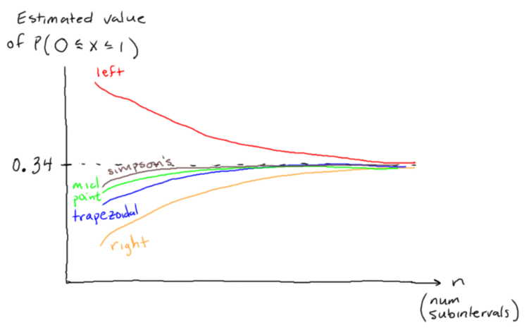
PART 2
Location: assignment-problems
Skim the following section of http://learnyouahaskell.com/starting-out.
Texas ranges I'm a list comprehension
Create Haskell file ComplicatedList.hs and write a function calcList in that takes an input number n and counts the number of ordered pairs [x,y] that satisfy $-n \leq x,y \leq n$ and $x-y \leq \dfrac{xy}{2} \leq x+y$ and $x,y \notin \{ -2, -1, 0, 1, 2 \}.$ This function should generate a list comprehension and then count the length of that list.
To check your function, print calcList 50. You should get a result of $16.$
PART 3
Complete these C++/Shell/SQL coding challenges and submit screenshots.
https://www.hackerrank.com/challenges/c-tutorial-for-loop/problem
https://www.hackerrank.com/challenges/c-tutorial-functions/problem
https://www.hackerrank.com/challenges/bash-tutorials---comparing-numbers/problem
https://www.hackerrank.com/challenges/bash-tutorials---more-on-conditionals/problem
https://sqlzoo.net/wiki/SELECT_within_SELECT_Tutorial (queries 4,5,6)
For C++/Shell, each screenshot should include your username, the problem title, and the "Status: Accepted" indicator.
For SQL, each screenshot should include the problem number, the successful smiley face, and your query.
Here's a helpful example of some bash syntax. (The spaces on the inside of the brackets are really important! It won't work if you remove the spaces, i.e.
[$n -gt 100])read n if [ $n -gt 100 ] || [ $n -lt -100 ] then echo What a large number. else echo The number is smol. if [ $n -eq 13 ] then echo And it\'s unlucky!!! fi fi
PART 4
a.
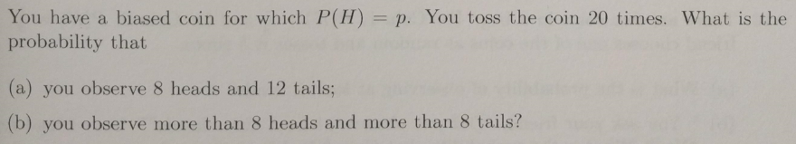
b.
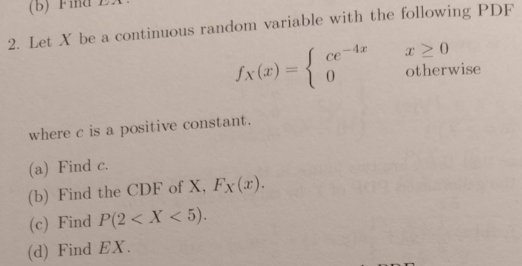
Remember that for a probability distribution $f(x),$ the cumulative distribution function (CDF) is $F(x) = P(X \leq x) = \displaystyle \int_{-\infty}^x f(x) \, \textrm dx.$
Remember that $EX$ means $\textrm E[X].$
Problem 45-3
Review; 10% of assignment grade; 15 minutes estimate
Commit your code to GitHub. When you submit your assignment, include a link to your commit(s). If you don't do this, your assignment will receive a grade of $0$ until you resubmit with links to your commits.
Additionally, do the following:
Make 2 GitHub issues on your assigned classmate's repository (but NOT
assignment-problems). See eurisko.us/resources/#code-reviews to determine your assigned classmate. When you submit your assignment, include the links to the issues you created.~Resolve an issue that has been made on your own GitHub repository. When you submit your assignment, include a link to the issue you resolved. (If you don't have any issues on any of your repositories, then you don't have to do anything, but state that this is the case when you turn in your assignment.)~ Let's actually hold off on this bit for the next couple weeks, so that we can build up an inventory of issues on our repositories. Then, once we have an inventory of 5-10 issues to choose from each time, we can start resolving them.
SUBMISSION TEMPLATE
For your submission, copy and paste your links into the following template:
Breadth-first and depth-first repl.it link: _____
Commit link for graph repo: _____
Repl.it link to Haskell code: _____
Commit link for assignment-problems repo: _____
Link to C++/SQL screenshots (Overleaf or Google Doc): _____
Link to probability solutions (on Overleaf): _____
Issue 1: _____
Issue 2: _____Problem 44-1
Primary problem; 45% of assignment grade; 75 minutes estimate
Location: Overleaf
a. Submit corrections to final (put your corrections in an overleaf doc). I made a final review video that goes through each problem, available here: https://vimeo.com/496684498
For each correction, explain
- what misunderstanding you had, and
- how you get to the correct result.
Important: The majority of the misunderstandings should NOT be "I ran out of time", and when you explain how to get to the correct result, SHOW ALL WORK.
b. A food manufacturing company is testing out some recipes for roast beef sandwiches and peanut butter sandwiches. They fed sandwiches to several subjects, and the subjects rated the sandwiches.
Slices of Roast Beef | Tablespoons of Peanut Butter | Rating |
--------------------------------------------------------------
0 | 0 | 1 |
1 | 0 | 2 |
2 | 0 | 4 |
4 | 0 | 8 |
6 | 0 | 9 |
0 | 2 | 2 |
0 | 4 | 5 |
0 | 6 | 7 |
0 | 8 | 6 |(i) Create a file machine-learning/analysis/sandwich_ratings.py where you use your linear regressor to fit the following model:
State this model in your Overleaf document.
(ii) Use your model to predict the rating of a sandwich with $5$ slices of roast beef and no peanut butter. State the prediction in your Overleaf document.
(iii) Use your model to predict the rating of a sandwich with $5$ slices of roast beef AND $5$ tablespoons of peanut butter (both ingredients on the same sandwich). State the prediction in your Overleaf document.
(iv) Look back at your answers to (ii) and (iii). One of these predictions can be trusted, while the other cannot. Which can be trusted, and why can it be trusted? Which cannot be trusted, and why can't it be trusted? Why is it possible for the model to give a prediction that can't be trusted?
Problem 44-2
Supplemental problems; 45% of assignment grade; 75 minutes estimate
PART 1
In your machine-learning repository, create a folder machine-learning/datasets/. Go to https://people.sc.fsu.edu/~jburkardt/data/csv/csv.html, download the file airtravel.csv, and put it in your datasets/ folder.
In Python, you can read a csv as follows:
>>> path_to_datasets = '/home/runner/machine-learning/datasets/'
>>> filename = 'airtravel.csv'
>>> with open(path_to_datasets + filename, "r") as file:
print(file.read())
"Month", "1958", "1959", "1960"
"JAN", 340, 360, 417
"FEB", 318, 342, 391
"MAR", 362, 406, 419
"APR", 348, 396, 461
"MAY", 363, 420, 472
"JUN", 435, 472, 535
"JUL", 491, 548, 622
"AUG", 505, 559, 606
"SEP", 404, 463, 508
"OCT", 359, 407, 461
"NOV", 310, 362, 390
"DEC", 337, 405, 432Write a @classmethod called DataFrame.from_csv(path_to_csv, header=True) that constructs a DataFrame from a csv file (similar to how DataFrame.from_array(arr) constructs the DataFrame from an array).
Test your method as follows:
>>> path_to_datasets = '/home/runner/machine-learning/datasets/'
>>> filename = 'airtravel.csv'
>>> filepath = path_to_datasets + filename
>>> df = DataFrame.from_csv(filepath, header=True)
>>> df.columns
['"Month"', '"1958"', '"1959"', '"1960"']
>>> df.to_array()
[['"JAN"', '340', '360', '417'],
['"FEB"', '318', '342', '391'],
['"MAR"', '362', '406', '419'],
['"APR"', '348', '396', '461'],
['"MAY"', '363', '420', '472'],
['"JUN"', '435', '472', '535'],
['"JUL"', '491', '548', '622'],
['"AUG"', '505', '559', '606'],
['"SEP"', '404', '463', '508'],
['"OCT"', '359', '407', '461'],
['"NOV"', '310', '362', '390'],
['"DEC"', '337', '405', '432']]PART 2
Location: assignment-problems
Skim the following section of http://learnyouahaskell.com/starting-out.
An intro to lists
Create Haskell file ListProcessing.hs and write a function prodFirstLast in Haskell that takes an input list arr and computes the product of the first and last elements of the list. Then, apply this function to the input [4,2,8,5].
Tip: use the !! operator and the length function.
Your file will look like this:
prodFirstLast arr = (your code here)
main = print (prodFirstLast [4,2,8,5])Note that, to print out an integer, we use print instead of putStrLn.
(You can also use print for most strings. The difference is that putStrLn can show non-ASCII characters like "я" whereas print cannot.)
Run your function and make sure it gives the desired output (which is 20).
PART 3
a. Complete these introductory C++ coding challenges and submit screenshots:
https://www.hackerrank.com/challenges/c-tutorial-basic-data-types/problem
https://www.hackerrank.com/challenges/c-tutorial-conditional-if-else/problem
b. Complete these Bash coding challenges and submit screenshots:
https://www.hackerrank.com/challenges/bash-tutorials---a-personalized-echo/problem
https://www.hackerrank.com/challenges/bash-tutorials---the-world-of-numbers/problem
(Each screenshot should include your username, the problem title, and the "Status: Accepted" indicator.)
c. Complete SQL queries 1-3 here and submit screenshots:
(Each screenshot should include the problem number, the successful smiley face, and your query.)
PART 4
a. As we will see in the near future, the standard normal distribution comes up A LOT in the context of statistics. It is defined as
$$ p(x) = \dfrac{1}{\sqrt{2\pi}} e^{-x^2/2}. $$The reason why we haven't encountered it until now is that it's difficult to integrate. In practice, it's common to use a pre-computed table of values to look up probabilities from this distribution.
The actual problem: Write a function calc_standard_normal_probability(a,b) to approximate $P(a \leq X \leq b)$ for the standard normal distribution, using a Riemann sum with step size 0.001.
To check your function, print out estimates of the following probabilities:
$P(-1 \leq x \leq 1)$
$P(-2 \leq x \leq 2)$
$P(-3 \leq x \leq 3)$
Your estimates should come out close to 0.68, 0.955, 0.997 respectively. (https://en.wikipedia.org/wiki/68%E2%80%9395%E2%80%9399.7_rule)
b.
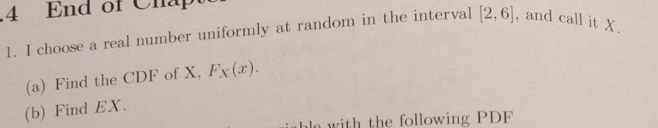
"CDF" stands for Cumulative Distribution Function. The CDF of a probability distribution $f(x)$ is defined as $$ F(x) = P(X \leq x) = \int_{-\infty}^x f(x) \, \textrm dx. $$
Your answer for the CDF will be a piecewise function (3 pieces).
$EX$ means $E[X].$
c.

Problem 44-3
Review; 10% of assignment grade; 15 minutes estimate
Commit your code to GitHub. When you submit your assignment, include a link to your commit(s). If you don't do this, your assignment will receive a grade of $0$ until you resubmit with links to your commits.
Additionally, do the following:
Make 2 GitHub issues on your assigned classmate's repository (but NOT
assignment-problems). See eurisko.us/resources/#code-reviews to determine your assigned classmate. When you submit your assignment, include the links to the issues you created.~Resolve an issue that has been made on your own GitHub repository. When you submit your assignment, include a link to the issue you resolved. (If you don't have any issues on any of your repositories, then you don't have to do anything, but state that this is the case when you turn in your assignment.)~ Let's actually hold off on this bit for the next couple weeks, so that we can build up an inventory of issues on our repositories. Then, once we have an inventory of 5-10 issues to choose from each time, we can start resolving them.
Problem 43-1
Primary problem; 40% of assignment grade; 60 minutes estimate
In your EulerEstimator, update the plot() method to work with systems of equations. (We wrote this method a while ago, but we've significantly refactored our estimator since then.)
Use the plot() method to plot the system from problem 40-2 on the interval $[0,5],$ using the initial condition $A(0) = B(0) = C(0) = 0$ and step size $\Delta t = 0.01.$
Starting at $t=0,$ step forward with a step size of $\Delta t = 0.01$ until you get to the value $t=5.$
Keep track of the values of the independent variable ($t$) and the dependent variables ($A,B,C$ in this case) as you step forward.
Using the values that you kept track of, plot the curves $y = A(t),$ $y = B(t),$ and $y = C(t)$ on the same graph. Make them different colors.
Once you've got a plot, post it on the #computation-and-modeling channel in Slack to compare with your classmates.
Problem 43-2
Supplemental problems; 50% of assignment grade; 75 minutes estimate
PART 1
Location: assignment-problems
Write a function random_draw(distribution) that draws a random number from the probability distribution. Assume that the distribution is an array such that distribution[i] represents the probability of drawing i.
Here are some examples:
random_draw([0.5, 0.5])will return0or1with equal probabilityrandom_draw([0.25, 0.25, 0.5])will return0a quarter of the time,1a quarter of the time, and2half of the timerandom_draw([0.05, 0.2, 0.15, 0.3, 0.1, 0.2])will return05% of the time,120% of the time,215% of the time,330% of the time,410% of the time, and0.220% of the time.
The way to implement this is to
- turn the distribution into a cumulative distribution,
- choose a random number between 0 and 1, and then
- find the index of the first value in the cumulative distribution that is greater than the random number.
Distribution:
[0.05, 0.2, 0.15, 0.3, 0.1, 0.2]
Cumulative distribution:
[0.05, 0.25, 0.4, 0.7, 0.8, 1.0]
Choose a random number between 0 and 1:
0.77431
The first value in the cumulative distribution that is
greater than 0.77431 is 0.8.
This corresponds to the index 4.
So, return 4.To test your function, generate 1000 random numbers from each distribution and ensure that their average is close to the true expected value of the distribution.
In other words, for each of the following distributions, print out the true expected value, and then print out the average of 1000 random samples.
[0.5, 0.5][0.25, 0.25, 0.5][0.05, 0.2, 0.15, 0.3, 0.1, 0.2]
PART 2
Location: assignment-problems
Skim the following sections of http://learnyouahaskell.com/starting-out.
- Ready, set, go!
- Baby's first functions
Create Haskell file ClassifyNumber.hs and write a function classifyNumber in Haskell that takes an input number x and returns
"negative"ifxis negative"nonnegative"ifxis nonnegative.
Then, apply this function to the input 5.
Your file will look like this:
classifyNumber x = (your code here)
main = putStrLn (classifyNumber 5)Now, run your function by typing the following into the command line:
>>> ghc --make ClassifyNumber
>>> ./ClassifyNumberghc is a Haskell compiler. It will compile or "make" an executable object using your .hs file. The command ./ClassifyNumber. actually runs your executable object.
PART 3
Complete this introductory C++ coding challenge: https://www.hackerrank.com/challenges/cpp-input-and-output/problem
Submit a screenshot that includes the name of the problem (top left), your username (top right), and Status: Accepted (bottom).

PART 4
Complete this introductory Shell coding challenge: https://www.hackerrank.com/challenges/bash-tutorials---looping-and-skipping/problem
The following example of a for loop will be helpful:
for i in {2..10}
do
((n = 5 * i))
echo $n
doneNote: You can solve this problem with just a single for loop
Again, submit a screenshot that includes the name of the problem (top left), your username (top right), and Status: Accepted (bottom), just like in part 3.
PART 5
Complete queries 11-14 here: https://sqlzoo.net/wiki/SELECT_from_Nobel_Tutorial
As usual, include a screenshot for each problem that includes the problem number, the successful smiley face, and your query.
PART 6
Location: Overleaf
Complete the following probability problems:
a.
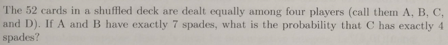
- Use conditional probability. In other words, compute the probability that C has exactly $4$ spaces, given that A and B have exactly 7 spaces (together).
b.
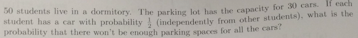
- Write your answer using sigma notation or "dot dot dot" notation.
Problem 43-3
Review; 10% of assignment grade; 15 minutes estimate
Commit your code to GitHub. When you submit your assignment, include a link to your commit(s). If you don't do this, your assignment will receive a grade of $0$ until you resubmit with links to your commits.
Additionally, do the following:
Make a GitHub issue on your assigned classmate's repository (but NOT
assignment-problems). See eurisko.us/resources/#code-reviews to determine your assigned classmate. When you submit your assignment, include a link to the issue you created.Resolve an issue that has been made on your own GitHub repository. When you submit your assignment, include a link to the issue you resolved. (If you don't have any issues on any of your repositories, then you don't have to do anything, but state that this is the case when you turn in your assignment.)
Problem 42-1
Estimated Time: 60 minutes
Grade Weighting: 50%
Complete SQL Zoo Modules 2 (all of it), and problems 1-10 in Module 3 (https://sqlzoo.net/). Put screenshots in an overleaf doc or submit them separately on Canvas (up to you).
Problem 42-2
Location: Overleaf
Estimated Time: 45 minutes
Grade Weighting: 50%
Complete the following probability problems, taken from Introduction to Probability: Statistics and Random Processes by Hossein Pishro-Nik:
a.
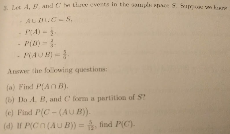
b.

- Remember that $\textrm{Var}[A + B] = \textrm{Var}[A] + \textrm{Var}[B] + 2 \textrm{Cov}[A,B].$
c.
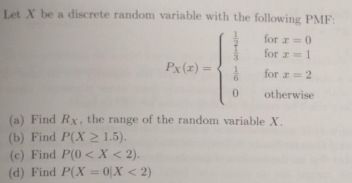
- Use Bayes' rule.
d.

Remember that PMF means "probability mass function". This is just the function $P(Z=z).$
Tip: Find the possible values of $Z,$ and then find the probabilities of those values of $Z$ occurring. Your answer will be a piecewise function: $$ P(z) = \begin{cases} \_\_\_, \, z=\_\_\_ \\ \_\_\_, \, z=\_\_\_ \\ \ldots \end{cases} $$
e.
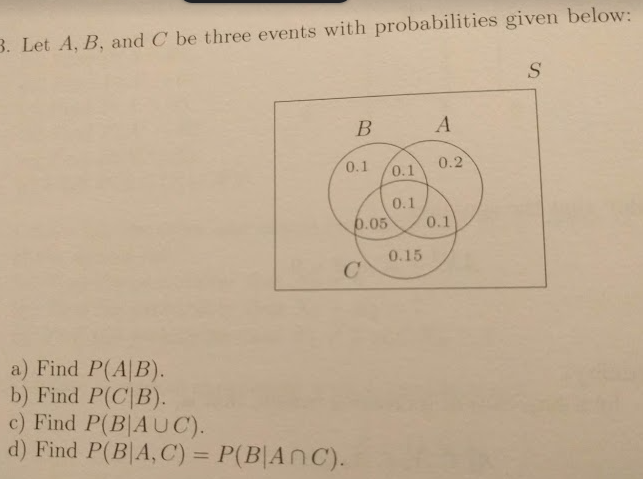
f.
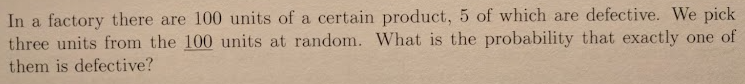
Problem 41-1
Wrapping up the semester...
- Turn in any missing assignments / resubmissions / quiz corrections by Sunday 1/3 at the very latest. Finish strong! I want to give out strong grades, but I can only do that if you're up to date with all your work and you've done it well.
Problem 41-2
Review for the final:
Basic probability
coin flipping, definitions of independent/disjoint, conditional probability, mean, variance, standard deviation, covariance, how variance/covariance are related to expectation
Probability distributions
identifying probability distributions, solving for an unknown constant so that a probability distribution is valid, discrete uniform, continuous uniform, exponential, poisson, using cumulative distributions i.e. P(a <= x < b) = P(x < b) - P(x < a), KL divergence, joint distributions, basic probability computations with joint distributions
Bayesian stats
likelihood distribution, posterior/prior distributions
Regression
pseudoinverse, fitting a linear regression, fitting a logistic regression, end behaviors of linear and logistic regression
Basic algorithms
Basic string processing (something like separate_into_words and reverse_word_order from Quiz 1), Implementing a recursive sequence, euler estimation, unlisting, converting between binary and decimal
Matrix algorithms
matrix multiplication, converting to reduced row echelon form, determinant using rref, determinant using cofactors, why determinant using rref is faster than determinant using cofactors, inverse via augmented matrix
Sorting algorithms
tally sort, merge sort (also know how to merge two sorted lists), swap sort
Optimization algorithms
Newton-Raphson (i.e. the “zero of tangent line” method), gradient descent, grid search (also know how to compute cartesian product)
Data structures
Linked list, tree, stack, queue
Object-oriented programming
Operator overloading, inheritance
Code quality & debugging
Naming conventions, be able to identify good vs bad variable names, be able to identify good vs bad github commits, know how often to make github commits, know the steps for debugging (i.e. print out stuff & use that to figure out where things are going wrong)
Problem 40-1
Estimated Time: 30 minutes
Location:
machine-learning/src/linear-regressor.py
machine-learning/tests/test_linear-regressor.py
Grading: 10 points
Extend your LinearRegressor to handle data points of any dimension. Assert that the following tests pass:
>>> df = DataFrame.from_array(
[[0, 0, 0.1],
[1, 0, 0.2],
[0, 2, 0.5],
[4,5,0.6]],
columns = ['scoops of chocolate', 'scoops of vanilla', 'taste rating']
)
>>> regressor = LinearRegressor(df, dependent_variable='taste rating')
>>> regressor.coefficients
{
'constant': 0.19252336,
'scoops of chocolate': -0.05981308,
'scoops of vanilla': 0.13271028
}
# these coefficients are rounded, you should only round
# in your assert statement
>>> regressor.predict({
'scoops of chocolate': 2,
'scoops of vanilla': 3
})
0.47102804Note: Your class should NOT be tailored to 3-dimensional data points. It should be data points to any number of dimensions.
Problem 40-2
Estimated Time: 90 minutes
Location:
simulation/src/euler_estimator.py
simulation/tests/test_euler_estimator.py
Grading: 10 points
Generalize your EulerEstimator to systems of differential equations. For example, we should be able to model the system
starting at the point $\left( t, \begin{bmatrix} A \\ B \\ C \end{bmatrix} \right) = \left( 0, \begin{bmatrix} 0 \\ 0 \\ 0 \end{bmatrix} \right)$ as follows:
>>> derivatives = {
'A': (lambda t,x: x['A'] + 1),
'B': (lambda t,x: x['A'] + x['B']),
'C': (lambda t,x: 2*x['B'])
}
>>> euler = EulerEstimator(derivatives = derivatives)
>>> initial_values = {'A': 0, 'B': 0, 'C': 0}
>>> initial_point = (0, initial_values)
>>> euler.calc_derivative_at_point(initial_point)
{'A': 1, 'B': 0, 'C': 0}
>>> point_2 = euler.step_forward(point = initial_point, step_size = 0.1)
>>> point_2
(0.1, {'A': 0.1, 'B': 0, 'C': 0})
>>> euler.calc_derivative_at_point(point_2)
{'A': 1.1, 'B': 0.1, 'C': 0}
>>> point_3 = euler.step_forward(point = point_2, step_size = -0.5)
>>> point_3
(-0.4, {'A': -0.45, 'B': -0.05, 'C': 0})
>>> euler.calc_estimated_points(point=point_3, step_size=2, num_steps=3)
[
(-0.4, {'A': -0.45, 'B': -0.05, 'C': 0}), # starting point
(1.6, {'A': 0.65, 'B': -1.05, 'C': -0.2)), # after 1st step
(3.6, {'A': 3.95, 'B': -1.85, 'C': -4.4)), # after 2nd step
(5.6, {'A': 13.85, 'B': 2.35, 'C': -11.8)) # after 3rd step
]Problem 39-1
Estimated time: 90 minutes
Grading: 15 points
Location: graph/src/tree.py
In this problem, you will start writing a class Tree that goes in a repository graph. (A tree is a special case of the more general concept of a graph.)
Your Tree class will take in a list of edges, and then the build_from_edges() method will connect up some Nodes with that arrangement of edges. It will be similar to LinkedList, but now a node can have more than one child.
The easiest way to build the tree is as follows:
- Look at the edges, identify the root, and create a node for the root.
- Look at the edges, identify the children of the root, create a node for each of them, and put that node in the root's
childrenattribute. - For each of those children, identify their children, create a node for each, and put that node in its parent's
childrenattribute. - Keep repeating this procedure until there are no more children to go through
The easiest way is to do a while loop: make a node_array that's initialized as node_array = [self.root], and while node_array is nonempty, do the following:
- loop through all nodes in that array, set their children, and put their children in a child_array
- Set
node_array = list(child_array).
>>> edges = [('a','c'), ('e','g'), ('e','i'), ('e','a'), ('g','b'), ('a','d'), ('d','f'), ('f','h'), ('d','j'), ('c','k')]
>>> tree = Tree(edges)
>>> tree.build_from_edges()
first, create the root node: e
e
then, create nodes for the children of e:
e has children a, i, g
e
/|\
a i g
then, create nodes for the children of a, i, g:
a has children c, d
i has no children
g has a child b
e
/|\
a i g
/| |
c d b
then, create nodes for the children of c, d, b:
c has a child k
d has children j and f
b has no children
e
/|\
a i g
/| |
c d b
| |\
k j f
then, create nodes for the children of k, j, f:
k has no children
j has no children
f has a child h
e
/|\
a i g
/| |
c d b
| |\
k j f
|
h
then, create nodes for the children of h:
h has no children
e
/|\
a i g
/| |
c d b
| |\
k j f
|
h
we've run out of children, so we're done
>>> tree.root.value
'e'
>>> [node.value for node in tree.root.children]
['a', 'i', 'g']
# you may need to change the output of this test (and future tests)
# for example, if you have ['g', 'i', 'a'], then that's fine
>>> [node.value for node in tree.root.children[0].children] # children of a
['c', 'd']
# you may need to change the output of this test (and future tests)
# for example, if you had ['g', 'i', 'a'] earlier, then the
# output would be the children of 'g', which is just ['b']
>>> [node.value for node in tree.root.children[1].children] # children of i
[]
>>> [node.value for node in tree.root.children[2].children] # children of g
['b']
>>> [node.value for node in tree.root.children[0].children[0].children] # children of c
['k']
>>> [node.value for node in tree.root.children[0].children[1].children] # children of d
['j', 'f']
>>> [node.value for node in tree.root.children[2].children[0].children] # children of b
[]
>>> [node.value for node in tree.root.children[0].children[0].children[0].children] # children of k
[]
>>> [node.value for node in tree.root.children[0].children[1].children[0].children] # children of j
[]
>>> [node.value for node in tree.root.children[0].children[1].children[1].children] # children of f
['h']
>>> [node.value for node in tree.root.children[0].children[1].children[1].children[0].children] # children of f
[]Problem 39-2
Estimated Time: 20 min
Location: Overleaf
Grading: 5 points
(Taken from Introduction to Probability: Statistics and Random Processes by Hossein Pishro-Nik)
a.
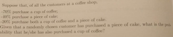
- Draw a Venn diagram and use Bayes' Theorem: $P(A \, | \, B) = \dfrac{P(A \textrm{ and } B)}{P(B)}$
b.
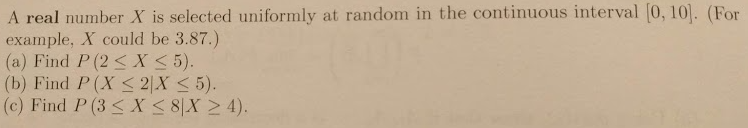
- Again, use Bayes' Theorem (but this time, you don't need a Venn diagram).
Problem 38-1
Estimated time: 90 minutes
Grading: 15 points
Location: Overleaf
a. Let $X,Y \sim p(x,y).$ Prove that $\textrm{E}[X+Y] = \textrm{E}[X] + \textrm{E}[Y].$
- Start with $\textrm{E}[X+Y],$ write the definition in terms of an integral, and then expand out that integral until it can be condensed into $\textrm{E}[X] + \textrm{E}[Y].$
b. The covariance of two random variables $X, Y$ is defined as
$$\text{Cov}[X, Y] = \text{E}[(X - \textrm{E}[X])(Y - \textrm{E}[Y])].$$Prove that
$$\text{Cov}[X,Y] = \textrm{E}[XY] - \textrm{E}[X] \textrm{E}[Y].$$- It will be fastest to multiply out the product and then expand out the result using part (a).
c. Given that $X \sim U[0,1],$ compute $\text{Cov}[X,X^2].$
It will be fastest to use the identity $\text{Cov}[X,Y] = E[XY] - E[X] E[Y].$
You should get a result of $\dfrac{1}{12}.$
d. Given that $X \sim \mathcal{U}[0,1],$ and $Y \sim \mathcal{U}[0,1],$ we have $(X,Y) \sim \mathcal{U}([0,1] \times [0,1]).$ Compute $\text{Cov}[X, Y].$
It will be fastest to use the identity $\text{Cov}[X,Y] = E[XY] - E[X] E[Y].$
You should get a result of $0.$ (It will always turn out that the covariance of independent random variables is zero.)
e. Prove that
$$\text{Var}[X + Y] = \text{Var}[X] + \text{Var}[Y] + 2 \text{Cov}[X,Y].$$You can use either of two methods.
Method 1: start with $\textrm{Var}[X+Y],$ write the definition in terms of an integral, and then expand out that integral until it can be condensed the desired result.
Method 2: start with $\textrm{Var}[X+Y],$ then use the identity $\textrm{Var}[A] = \textrm{E}[A^2] - \textrm{E}[A]^2,$ and then use parts (a) and (d).
Problem 38-2
Estimated Time: 30 min
Location: Overleaf
Grading: 5 points
- Complete Module 8 of Sololearn's C++ Course. Take a screenshot of the completed module, with your user profile showing, and submit it along with the assignment.
Problem 37-1
Estimated time: 30 minutes
Grading: 10 points
Location: assignment-problems/tree.py
Write functions get_children, get_parents, and get_roots. Assert that they pass the following tests. Remember that to find the root of the tree, you can just look for the node that has no parents.
>>> edges = [('a','c'), ('e','g'), ('e','i'), ('e','a'), ('d','b'), ('a','d'), ('d','f'), ('f','h'), ('d','j'), ('d','k')]
represents this tree:
e
/|\
a i g
/|
c d
/|\\
b j fk
|
h
>>> get_children('e', edges)
['a', 'i', 'g'] # note: the order here doesn't matter -- you can have the
# children in any order
>>> get_children('c', edges)
[]
>>> get_children('f', edges)
['h']
>>> get_parents('e', edges)
[]
>>> get_parents('c', edges)
['a']
>>> get_parents('f', edges)
['d']
>>> get_roots(edges)
['e']Problem 37-2
Estimated time: 30 minutes
Grading: 10 points
Location: Overleaf
a. Fit a linear regression $y=\beta_0 + \beta_1 x_1 + \beta_2 x_2$ to the following dataset, where points take the form $(x_1, x_2, y).$ This will be the same process as usual, using the pseudoinverse. Show all the steps in your work.
points = [(0, 0, 0.1), (1, 0, 0.2), (0, 2, 0.5), (4,5,0.6)]b. Fit a logistic regression $y=\dfrac{1}{1+e^{\beta_0 + \beta_1 x_1 + \beta_2 x_2} }$ to the same dataset. Again, show all the steps in your work.
Problem 37-3
Estimated time: 30 minutes
Grading: 10 points
Location: Overleaf
Consider the joint exponential distribution defined by
$$p(x,y) = \begin{cases} k e^{-2 x - 3 y} & x,y \geq 0 \\ 0 & x<0 \text{ or } y < 0 \end{cases}.$$a. Find the value of $k$ such that $p(x,y)$ is a valid probability distribution.
b. Given that $(X,Y) \sim p,$ compute $\text{E}[X]$ and $\text{E}[Y].$
c. Given that $(X,Y) \sim p,$ compute $\text{Var}[X]$ and $\text{Var}[Y].$
d. Given that $(X,Y) \sim p,$ compute $P\left( X < 4, \, Y < 5 \right).$ Write your answer in terms of $e,$ in simplest form.
Problem 36-1
Estimated time: 45 minutes
Grading: 10 points
Location: Overleaf
Suppose you are a mission control analyst who is looking down at an enemy headquarters through a satellite view, and you want to get an estimate of how many tanks they have. Most of the headquarters is hidden, but you notice that near the entrance, there are four tanks visible, and these tanks are labeled with the numbers $52, 30, 68, 7.$ So, you assume that they have $N$ tanks that they have labeled with numbers from $1$ to $N.$
Your commander asks you for an estimate: with $95\%$ certainty, what's the max number of tanks they have?
In this problem, you'll answer that question using the same process that you used in 35-1 (a,b,f). In your answer, show your work and justify every step of the way.
Problem 36-2
Estimated time: 45 minutes
Grading: 10 points
Location: assignment-problems/grid_search.py
Write a function grid_search(objective_function, grid_lines) that takes the Cartesian product of the grid_lines in the search space, evaluates the objective_function at all points of intersection, and returns the point where the objective_function takes the lowest value.
Assert that it passes the following test:
>>> def two_variable_function(x, y):
return (x-1)**2 + (y-1)**3
>>> x_lines = [0, 0.25, 0.75]
>>> y_lines = [0.9, 1, 1.1, 1.2]
>>> grid_lines = [x_lines, y_lines]
>>> grid_search(two_variable_function, grid_lines)
[0.75, 0.9]
Note: behind the scenes, grid_search is computing all
intersections of x_lines with y_lines to get the following
points:
[0, 0.9], [0, 1], [0, 1.1], [0, 1.2]
[0.25, 0.9], [0.25, 1], [0.25, 1.1], [0.25, 1.2]
[0.75, 0.9], [0.75, 1], [0.75, 1.1], [0.75, 1.2]
Then, it evaluates the function at these points and returns
the point that gave the lowest value.Problem 35-1
Estimated Time: 60 minutes
Locations: Overleaf AND assignment-problems/assignment_35_stats.py
Grading: 10 points
In this problem, you will perform another round of Bayesian inference, but this time on a different distribution. It will be very similar to Problem 27-3.
Your friend is randomly stating positive integers that are less than some upper bound (which your friend knows, but you don't know). The numbers your friend states are as follows:
1, 17, 8, 25, 3
You assume that the numbers come from a discrete uniform distribution $U\left\{1,2,\ldots,k\right\}$ defined as follows:
$$p_k(x) = \begin{cases} \dfrac{1}{k} & x \in \left\{1,2,\ldots,k\right\} \\ 0 & x \not\in \left\{1,2,\ldots,k\right\} \end{cases}$$a. Compute the likelihood $P(\left\{ 1, 17, 8, 25, 3 \right\} | \, k).$ Remember that the likelihood is just the probability of getting the result $ \left\{ 1, 17, 8, 25, 3 \right\}$ under the assumption that the data was sampled from the distribution $p_k(x).$ Your answer should be a piecewise function expressed in terms of $k\mathbin{:}$
$$P(\left\{ 1, 17, 8, 25, 3 \right\} | \, k) = \begin{cases} \_\_\_ & k \geq \_\_\_ \\ 0 & \textrm{otherwise} \end{cases}$$- Note: To figure out the $k \geq \_\_\_$ part, keep in mind that the data $\left\{ 1, 17, 8, 25, 3 \right\}$ is drawn from $\left\{ 1, 2, \ldots, k \right\}.$
b. Compute the posterior distribution by normalizing the likelihood. That is to say, find the constant $c$ such that $$\sum_{k=1}^\infty c \cdot P(\left\{ 1, 17, 8, 25, 3 \right\} | \, k) = 1.$$ Then, the posterior distribution will be $$P(k \, | \left\{ 1, 17, 8, 25, 3 \right\})= c \cdot P(\left\{ 1, 17, 8, 25, 3 \right\} \, | \, k).$$
- SUPER IMPORTANT: You won't be able to figure this out analytically (i.e. just using pen and paper). Instead, you should write a Python script in
assignment-problems/assignment_35_stats.pyto approximate the sum by evaluating it for a very large number of terms. You should use as many terms as you need until the result appears to converge.
c. What is the most probable value of $k?$ You can tell this just by looking at the distribution $P(k \, | \left\{ 1, 17, 8, 25, 3 \right\}),$ but make sure to justify your answer with an explanation.
d. The largest number in the dataset is $25.$ What is the probability that $25$ is actually the upper bound chosen by your friend?
e. What is the probability that the upper bound is less than or equal to $30?$
f. Fill in the blank: you can be $95\%$ sure that the upper bound is less than $\_\_\_.$
- SUPER IMPORTANT: You won't be able to figure this out analytically (i.e. just using pen and paper). Instead, you should write another Python function in
assignment-problems/assignment_35_stats.pyto approximate value of $k$ needed (i.e. the number of terms needed) to have $P(K \leq k \, | \left\{ 1, 17, 8, 25, 3 \right\}) = 0.95.$
Problem 35-2
Estimated Time: 30 minutes
Location: Overleaf
Grading: 5 points
A joint distribution is a probability distribution on two or more random variables. To work with joint distributions, you will need to use multi-dimensional integrals.
For example, given a joint distribution $p(x,y),$ the distribution must satisfy
$$ \begin{align*} \displaystyle \int_{-\infty}^\infty \int_{-\infty}^\infty p(x,y) \, \text{d}x \, \text{d}y = 1. \end{align*} $$The probability that $(X,Y) \in [a,b] \times [c,d]$ is given by
$$ \begin{align*} P((X,Y) \in [a,b] \times [c,d]) = \displaystyle \iint_{[a,b] \times [c,d]} p(x,y) \, \text{d}A, \end{align*} $$or equivalently,
$$ \begin{align*} P(a < X \leq b, \, c < Y \leq d) = \displaystyle \int_c^d \int_a^b p(x,y) \, \text{d}x \, \text{d}y. \end{align*} $$The expectations are
$$ \begin{align*} \textrm{E}[X] &= \displaystyle \int_c^d \int_a^b x \cdot p(x,y) \, \text{d}x \, \text{d}y, \\ \textrm{E}[Y] &= \displaystyle \int_c^d \int_a^b y \cdot p(x,y) \, \text{d}x \, \text{d}y. \end{align*} $$The joint uniform distribution $\mathcal{U}([a,b]\times[c,d])$ is a distribution such that all points $(x,y)$ have equal probability in the region $[a,b]\times[c,d]$ and zero probability elsewhere. So, it takes the form
$$p(x,y) = \begin{cases} k & (x,y) \in [a,b] \times [c,d] \\ 0 & (x,y) \not\in [a,b] \times [c,d] \end{cases}$$for some constant $k.$
a. Find the value of $k$ such that $p(x,y)$ is a valid probability distribution. Your answer should be in terms of $a,b,c,d.$
b. Given that $(X,Y) \sim p,$ compute $\text{E}[X]$ and $\text{E}[Y].$ You should get $\text{E}[X] = \dfrac{a+b}{2}$ and $\text{E}[Y] = \dfrac{c+d}{2}$
c. Geometrically, $[a,b] \times [c,d]$ represents a rectangle bounded by $x=a,$ $x=b,$ $y=c,$ and $y=d.$ What is the geometric interpretation of the point $(\text{E}[X], \text{E}[Y])$ in this rectangle?
Problem 34-1
Location: assignment-problems/cartesian_product.py
Estimated Time: 45 minutes
Grading: 10 points
Write a function cartesian_product(arrays) that computes the Cartesian product of all the lists in arrays.
>>> cartesian_product([['a'], [1,2,3], ['Y','Z']])
[['a',1,'Y'], ['a',1,'Z'], ['a',2,'Y'], ['a',2,'Z'], ['a',3,'Y'], ['a',3,'Z']]NOTE: This is a reasonably short function if you use the following procedure. You'll probably have to think a bit in order to get the implementation correct, though. (Make sure to post for help if you get stuck!)
Create a variable
pointsthat will be a list of all the points in the cartesian product. Initially, setpointsto consist of a single empty point:points = [[]].For each array in the input, create a new list of points.
The new set of points can be constructed by looping through each existing point and, for each existing point, adding several new points.
- For a given point, the new points can be constructed by appending each element of the array onto a copy of the given point.
Return the list of points.
Worked Example:
arrays = [['a'], [1,2,3], ['Y','Z']]
points: [[]]
considering array ['a']
considering element 'a'
new point ['a']
points: [['a']]
considering array [1,2,3]
considering element 1
new point ['a',1]
considering element 2
new point ['a',2]
considering element 3
new point ['a',3]
points: [['a',1], ['a',2], ['a',3]]
considering array ['Y','Z']
considering element 'Y'
new points ['a',1,'Y'], ['a',2,'Y'], ['a',3,'Y']
considering element 'Z'
new points ['a',1,'Z'], ['a',2,'Z'], ['a',3,'Z']
points: [[1,'a','Y'], [1,'a','Z'], [1,'b','Y'], [1,'b','Z'], [1,'c','Y'], [1,'c','Z']]Watch out! If you write new_point = old_point, then this just makes it so that new_point refers to old_point. So then whenever you change one of those variables, the other will change as well.
To actually make a separate independent copy, you can use new_point = list(old_point). That way, when you change one of the variables, it will have no effect on the other.
Problem 34-2
Locations:
machine-learning/src/gradient_descent.py
machine-learning/tests/test_gradient_descent.py
Estimated Time: 60 minutes
Grading: 10 points
Write a class GradientDescent that performs gradient descent on an input function with any number of arguments. This builds on top of Problem 25-1.
Tip: if you have a function
f(x,y,z)and a listargs = [0,5,3], then you can passf(*args)to evaluatef(0,5,3).**Tip: to get the number of variables that a function accepts as input, use
f.__code__.co_argcount. For example:>>> def f(x,y): return x**2 + y**2 >>> f.__code__.co_argcount 2
Assert that your GradientDescent passses the following tests. (Make sure to post for help if you get stuck!)
Note: the tests below are shown rounded to 3 decimal places. You should do the rounding in your assert statement, NOT in your GradientDescent class.
>>> def single_variable_function(x):
return (x-1)**2
>>> def two_variable_function(x, y):
return (x-1)**2 + (y-1)**3
>>> def three_variable_function(x, y, z):
return (x-1)**2 + (y-1)**3 + (z-1)**4
>>> def six_variable_function(x1, x2, x3, x4, x5, x6):
return (x1-1)**2 + (x2-1)**3 + (x3-1)**4 + x4 + 2*x5 + 3*x6
>>> minimizer = GradientDescent(f=single_variable_function, initial_point=[0])
>>> minimizer.point
[0]
>>> ans = minimizer.compute_gradient(delta=0.01)
[-2.000] # rounded to 5 decimal places
>>> minimizer.descend(alpha=0.001, delta=0.01, num_steps=1)
>>> minimizer.point
[0.002]
>>> minimizer = GradientDescent(f=two_variable_function, initial_point=[0,0])
>>> minimizer.point
[0,0]
>>> minimizer.compute_gradient(delta=0.01)
[-2.000, 3.000]
>>> minimizer.descend(alpha=0.001, delta=0.01, num_steps=1)
>>> minimizer.point
[0.002, -0.003]
>>> minimizer = GradientDescent(f=three_variable_function, initial_point=[0,0,0])
>>> minimizer.point
[0,0,0]
>>> minimizer.compute_gradient(delta=0.01)
[-2.000, 3.000, -4.000]
>>> minimizer.descend(alpha=0.001, delta=0.01, num_steps=1)
>>> minimizer.point
[0.002, -0.003, 0.004]
>>> minimizer = GradientDescent(f=six_variable_function, initial_point=[0,0,0,0,0,0])
>>> minimizer.point
[0,0,0,0,0,0]
>>> minimizer.compute_gradient(delta=0.01)
[-2.000, 3.000, -4.000, 1.000, 2.000, 3.000]
>>> minimizer.descend(alpha=0.001, delta=0.01, num_steps=1)
>>> minimizer.point
[0.002, -0.003, 0.004, -0.001, -0.002, -0.003]Make sure to push your finished code to Github with a commit message that says what you added/changed (you should always commit your code to Github after an assignment).
Problem 34-3
Estimated Time: 60 min
Location: Overleaf
Grading: 10 points
Complete Module 7 of Sololearn's C++ Course. Take screenshots of the completed modules, with your user profile showing, and submit them along with the assignment.
Complete queries 1-15 in Module 1 of the SQL Zoo. Here's a reference for the LIKE operator, which will come in handy.
Take a screenshot of each successful query and put them in an overleaf doc. When a query is successful, you'll see a smiley face appear. Your screenshots should look like this:
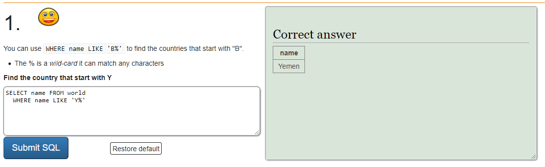
Problem 34-4
Take a look at all your assignments so far in this course. If there are any assignments with low grades, that you haven't already resubmitted, then be sure to resubmit them.
Also, if you haven't already, submit quiz corrections for all of the quizzes we've had so far!
Problem 33-1
Location: Overleaf
Estimated Time: 60 minutes
Grading: 10 points
Suppose you are again given the following dataset:
data = [(1,0.2), (2,0.25), (3,0.5)]Fit a logistic regression model $y=\dfrac{1}{1+e^{ax+b}}$ by hand.
- Re-express the model in the form $ax+b = \text{some function of }y$ (i.e. isolate $ax+b$ in the logistic regression model). Hint: your function of $y$ will involve $\ln.$
- Set up a system of equations and turn the system into a matrix equation.
- Find the best approximation to the solution of that matrix equation by using the pseudoinverse.
- Substituting your solution for the coefficients of the model, and plot the model along with the 3 given data points on the same graph to ensure that the model fits the data points well.
Show all of your steps. No code allowed in steps 1, 2, and 3! But in step 4, you can write a Python script for the final plot (or make the plot in latex).
Note: To plot points on a graph in Python, you can use the following:
plt.plot([1, 2, 3, 4], [1, 4, 9, 16]) # plot line segments
plt.plot([1, 2, 3, 4], [1, 4, 9, 16], 'ro') # plot red ('r') circles ('o')import matplotlib.pyplot as plt
plt.plot([1, 2, 3, 4], [1, 4, 9, 16], 'ro') # plot red ('r') circles ('o')

Problem 33-2
Location: Overleaf
Estimated Time: 30 minutes
Grading: 6 points
a. (2 points) Given that $X \sim p(x),$ where $p(x)$ is a continuous distribution, prove that for any real number $a$ we have $E[aX] = aE[X].$
- You should start by writing $E[aX]$ as an integral, manipulating it, and then simplifying the result into $aE[X].$ The manipulation will just be 1 step.
b. (4 points) Given that $X \sim p(x)$ where $p(x)$ is a continuous probability distribution, prove the identity $\text{Var}[X] = E[X^2] - E[X]^2.$
Problem 33-3
Estimated Time: 15 min
Grading: 4 points
- Complete Module 6 of Sololearn's C++ Course. Take a screenshot of the completed module, with your user profile showing, and submit it along with the assignment.
Problem 32-1
Estimated time: 60 min
Grading: 15 points
Locations:
machine-learning/src/linear_regressor.py
machine-learning/tests/test_linear_regressor.py
Create a class LinearRegressor that works as follows. Make sure your code is general. In other words, do not assume the dataset always consists of 3 points, do not assume the independent variable is always named 'progress', etc.
>>> df = DataFrame.from_array(
[[1,0.2],
[2,0.25],
[3,0.5]],
columns = ['hours worked', 'progress']
)
>>> regressor = LinearRegressor(df, dependent_variable='progress')
>>> regressor.coefficients
[0.01667, 0.15] # meaning that the model is progress = 0.01667 + 0.15 * (hours worked)
# these coefficients are rounded, but you should not round except for
# in your assert statement
>>> regressor.predict({'hours worked': 4})
0.61667Problem 32-2
Estimated Time: 15 min
Grading: 5 points
(Taken from Introduction to Probability: Statistics and Random Processes by Hossein Pishro-Nik)
a.
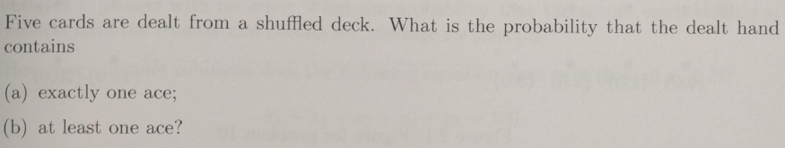
- Tip: for (b), compute $1-P(\textrm{complement}).$ Here, the complement is the event that you get no aces.
b.

- Tip: again, compute $1-P(\textrm{complement}).$
Problem 32-3
Estimated Time: 30 min
Grading: 10 points
Complete Module 5 of Sololearn's C++ Course. Take a screenshot of each completed module, with your user profile showing, and submit both screenshots along with the assignment.
Complete Module 4 of Sololearn's SQL Course. Take a screenshot of the completed module, with your user profile showing, and submit it along with the assignment.
Problem 31-1
Estimated Time: 60 min
Grading: 20 points
a.
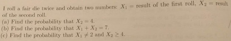
- Just count up the number of outcomes in favor, and divide by the total number of possible outcomes
b.
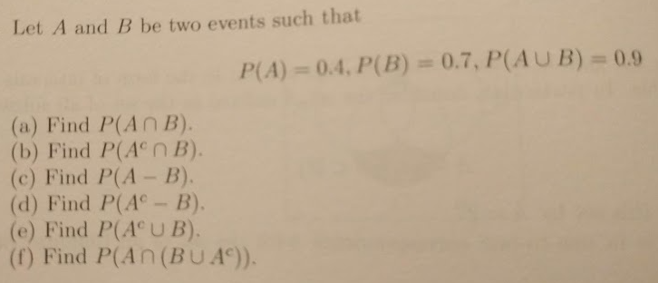
Remember that $A^C$ is the "complement" of $A,$ meaning all the space that is NOT included in $A.$
Remember that $A - B = \{ a \in A \, | \, a \not \in B \}.$ For example, $\{ 1, 2, 3 \} - \{2, 4, 6 \} = \{ 1, 3 \}.$
c.
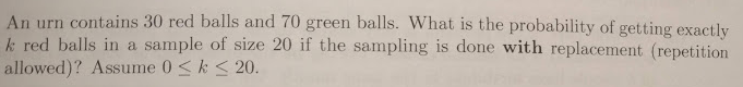
"With replacement" means that each time a ball is drawn, it is put back in for the next draw. So, it would be possible to draw the same ball more than once.
Multiply the following: (number of ways to choose k red balls in a sample of 20) $\times$ (probability of getting k red balls in a row) $\times$ (probability of getting 20-k green balls in a row)
This is very similar to flipping a biased coin, if you think of "red ball" as "heads" and "green ball" as "tails": (number of ways to get k heads in 20 flips) $\times$ (probability of getting k heads in a row) $\times$ (probability of getting 20-k tails in a row)
d.
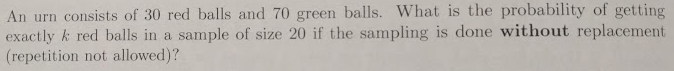
"Without replacement" means that each time a ball is drawn, it is NOT put back in for the next draw. So, it would NOT be possible to draw the same ball more than once.
It's easiest to do this problem if you think of just counting up the number of possibilities in favor, and dividing by the total number of possibilities.
Possibilities in favor: (number of ways to choose k of the 30 red balls) $\times$ (number of ways to choose 20-k of the 70 green balls)
Total number of possibilities: (number of ways to choose 20 of the 100 balls)
e.
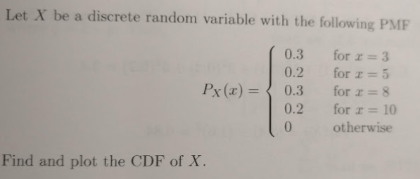
CDF stands for "Cumulative Distribution Function" and is defined as $\textrm{CDF}(x) = P(X \leq x).$
For example, $\textrm{CDF}(6) = P(X \leq 6) = 0.3 + 0.2 = 0.5.$
You're just plotting the function $y=\textrm{CDF}(x).$ You can just draw a picture and put it in your Overleaf doc as an image.
Problem 31-2
Estimated Time: 30 min
Grading: 10 points
Complete Module 4 of Sololearn's C++ Course. Take a screenshot of each completed module, with your user profile showing, and submit both screenshots along with the assignment.
Complete Module 3 of Sololearn's SQL Course. Take a screenshot of the completed module, with your user profile showing, and submit it along with the assignment.
Problem 30-1
Grading: 10 points
(Taken from Introduction to Probability: Statistics and Random Processes by Hossein Pishro-Nik)
a.
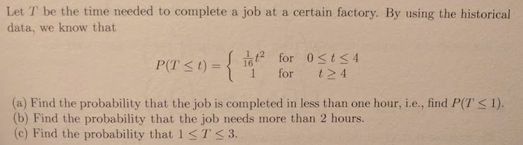
b.
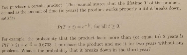
- Check: you should get a result of $0.1813.$ If you get stuck, then here's a link to a similar example, worked out.
c.
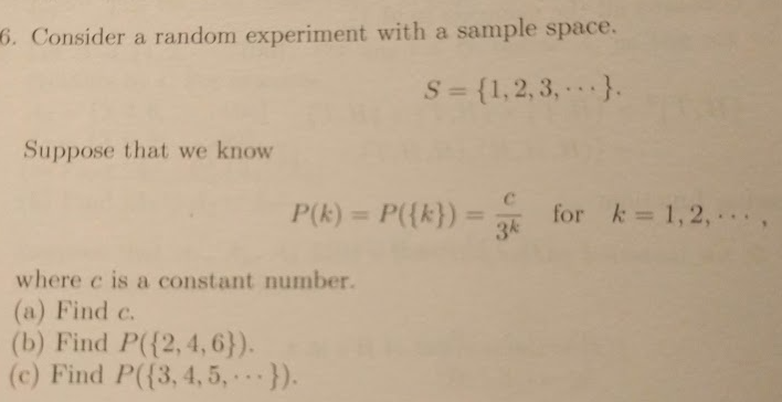
Problem 30-2
Location: assignment-problems/doubly_linked_list.py
Grading: 10 points
Create a class DoublyLinkedList that is similar to LinkedList, except that each Node has an additional attribute, prev, which returns the previous node. (It is the opposite of the next attribute.)
Make sure that prev is updated correctly in each of the operations.
Assert that the following test passes:
>>> doubly_linked_list = DoublyLinkedList('a')
>>> doubly_linked_list.append('c')
>>> doubly_linked_list.append('d')
>>> doubly_linked_list.append('e')
>>> doubly_linked_list.insert('b',1)
>>> doubly_linked_list.delete(3)
Note: at this point, the list looks like this:
a <--> b <--> c <--> e
>>> current_node = doubly_linked_list.get_node(3)
>>> node_values = [current_node.data]
>>> for _ in range(3):
current_node = current_node.prev
node_values.append(current_node.data)
>>> node_values
['e', 'c', 'b', 'a']Problem 30-3
Grading: 10 points
Complete Module 3 of Sololearn's C++ Course. Take a screenshot of each completed module, with your user profile showing, and submit both screenshots along with the assignment.
Complete Module 2 of Sololearn's SQL Course. Take a screenshot of the completed module, with your user profile showing, and submit it along with the assignment.
Problem 29-1
Location: Overleaf
Grading: 10 points
The Poisson distribution can be used to model how many times an event will occur within some continuous interval of time, given that occurrences of an event are independent of one another.
Its probability function is given by \begin{align*} p_\lambda(n) = \dfrac{\lambda^n e^{-\lambda}}{n!}, \quad n \in \left\{ 0, 1, 2, \ldots \right\}, \end{align*}
where $\lambda$ is the mean number of events that occur in the particular time interval.
SUPER IMPORTANT: Manipulating the Poisson distribution involves using infinite sums. However, these sums can be easily expressed using the Maclaurin series for $e^x\mathbin{:}$
\begin{align*} e^x = 1 + x + \dfrac{x^2}{2!} + \dfrac{x^3}{3!} + \ldots \end{align*}a. Consider the Poisson distribution defined by $$p_2(n) = \dfrac{2^n e^{-2}}{n!}.$$ Show that this is a valid probability distribution, i.e. all the probability sums to $1.$
b. Given that $N \sim p_2,$ compute $P(10 < N \leq 12).$ Leave your answer in exact form, and don't expand out the factorials. Pay close attention to the "less than" vs "less than or equal to" symbols.
c. Given that $N \sim p_2,$ compute $E[N].$
Using the Maclaurin series for $e^x,$ your answer should simplify to $2.$
When doing your series manipulations, don't use sigma notation. Instead, write out the first several terms of the series, followed by "dot dot dot", as shown in the Maclaurin series under the "SUPER IMPORTANT" label.
d. Given that $N \sim p_2,$ compute $\text{Var}[N].$ Using the Maclaurin series for $e^x,$ your answer should come out to a nice clean integer.
Using the Maclaurin series for $e^x,$ your answer should again simplify to $2.$
Again, when doing your series manipulations, don't use sigma notation. Instead, write out the first several terms of the series, followed by "dot dot dot", as shown in the Maclaurin series under the "SUPER IMPORTANT" label.
Tip: try multiplying out the binomial before you expand out the sums. Those 3 sums will be easier to compute, individually $$\begin{align*} e^{-2} \sum_{n=0}^\infty (n-2)^2 \dfrac{2^n}{n!} = e^{-2} \sum_{n=0}^\infty n^2 \cdot \dfrac{2^n}{n!} - e^{-2} \sum_{n=0}^\infty 4n \cdot \dfrac{2^n}{n!} + e^{-2} \sum_{n=0}^\infty 4 \cdot \dfrac{2^n}{n!} \end{align*}$$
Problem 29-2
Location: machine-learning/tests/test_data_frame.py
Grading: 10 points
Implement the following functionality in your DataFrame, and assert that these tests pass.
a. Loading an array. You'll need to use @classmethod for this one (read about it here).
>>> columns = ['firstname', 'lastname', 'age']
>>> arr = [['Kevin', 'Fray', 5],
['Charles', 'Trapp', 17],
['Anna', 'Smith', 13],
['Sylvia', 'Mendez', 9]]
>>> df = DataFrame.from_array(arr, columns)b. Selecting rows which satisfy a particular condition (given as a lambda function)
>>> df.select_rows_where(
lambda row: len(row['firstname']) >= len(row['lastname'])
and row['age'] > 10
).to_array()
[['Charles', 'Trapp', 17]]- Note: It's true that if you're just working with a plain old array, you can't do stuff like
row['firstname']. But we're working with a DataFrame class, which means we've got some creative freedom. You'll have to find way to convert a row array to a row dictionary, behind the scenes. In other words, make a functionconvert_row_from_array_to_dictthat takes a row['Kevin', 'Fray', 5]and converts it to
before you apply the lambda function.{ 'firstname': 'Kevin', 'lastname': 'Fray', 'age': 5 }
c. Ordering the rows by given column
>>> df.order_by('age', ascending=True).to_array()
[['Kevin', 'Fray', 5],
['Sylvia', 'Mendez', 9],
['Anna', 'Smith', 13],
['Charles', 'Trapp', 17]]
>>> df.order_by('firstname', ascending=False).to_array()
[['Sylvia', 'Mendez', 9],
['Kevin', 'Fray', 5],
['Charles', 'Trapp', 17],
['Anna', 'Smith', 13]]Problem 29-3
Grading: 5 points
Complete Module 1 of Sololearn's SQL Course. Take a screenshot of the completed module, with your user profile showing, and submit it along with the assignment.
Problem 28-1
Location: Overleaf
Grading: 10 points
Suppose you are given the following dataset:
data = [(1,0.2), (2,0.25), (3,0.5)]Fit a linear regression model $y=a+bx$ by hand by
- setting up a system of equations,
- turning the system into a matrix equation,
- finding the best approximation to the solution of that matrix equation by using the pseudoinverse, and
- substituting your solution for the coefficients of the model.
Show all of your steps. No code allowed!
Problem 28-2
Grading: 5 points
Create an apply method in your DataFrame, that passes the following test:
>>> data_dict = {
'Pete': [1, 0, 1, 0],
'John': [2, 1, 0, 2],
'Sarah': [3, 1, 4, 0]
}
>>> df1 = DataFrame(data_dict, column_order = ['Pete', 'John', 'Sarah'])
>>> df2 = df1.apply('John', lambda x: 7 * x)
>>> df2.data_dict
{
'Pete': [1, 0, 1, 0],
'John': [14, 7, 0, 14],
'Sarah': [3, 1, 4, 0]
}Problem 28-3
Location: Overleaf
Grading: 5 points
If you didn't get 100% on problem 27-3, revise it and submit it again on this assignment. If you already got 100%, then these 5 points are free.
Problem 28-4
Grading: 5 points
Complete Module 1 AND Module 2 of Sololearn's C++ Course. Take a screenshot of each completed module, with your user profile showing, and submit both screenshots along with the assignment.


Problem 27-1
Grading: 2 points
In your Matrix class, overload __rmul__and __pow__ so that you pass the following tests:
>>> A = Matrix([[1, 1, 0],
[2, -1, 0],
[0, 0, 3]])
>>> B = 0.1 * A
>>> B.elements
[[0.1, 0.1, 0],
[0.2, -0.1, 0],
[0, 0, 0.3]]
>>> C = A**3
>>> C.elements
[[3, 3, 0],
[6, -3, 0],
[0, 0, 27]]Problem 27-2
Grading: 5 points
Update EulerEstimator to make plots:
>>> euler = EulerEstimator(derivative = lambda t: t+1)
>>> euler.plot(point=(-5,10), step_size=0.1, num_steps=100)
for this example, the plot should look like the parabola
y = 0.5x^2 + x + 2.5
on the domain -5 <= x <= 5Problem 27-3
Location: Overleaf
Grading: 10 points
Suppose you toss a coin $10$ times and get the result $\text{HHHHT HHHHH}.$ From this result, you estimate that the coin is biased and generally lands on heads $90\%$ of the time. But how sure can you be? Let's quantify it.
a. Compute the likelihood $P(\text{HHHHT HHHHH}\, | \, k)$ where $P(H)=k.$ Remember that the likelihood is just the probability of getting the result $\text{HHHHT HHHHH}$ under the assumption that $P(H)=k.$ Your answer should be expressed in terms of $k.$
b. The likelihood $P(\text{HHHHT HHHHH} \, | \, k)$ can almost be interpreted as a probability distribution for $k.$ The only problem is that it doesn't integrate to $1.$
Create a probability distribution $P(k \, | \, \text{HHHHT HHHHH})$ that is proportional to the likelihood $P(\text{HHHHT HHHHH} \, | \, k).$ In other words, find the function $P(k)$ such that
$$ P(k \, | \, \text{HHHHT HHHHH}) = c \cdot P(\text{HHHHT HHHHH} \, | \, k) $$for some constant $c,$ and $\displaystyle \int_0^1 P(k \, | \, \text{HHHHT HHHHH}) = 1.$
Note: the distribution $P(k \, | \, \text{HHHHT HHHHH})$ is called the "posterior" distribution because it represents the probability distribution of $k$ after we have observed the event $\text{HHHHT HHHHH}.$
The probability distribution of $k$ before we observed the event is called the "prior" distribution and in this case was given by $P(k) \sim \mathcal{U}[0,1]$ since we did not know anything about whether or not the coin is biased (or how biased it is).
c. Using the prior distribution $P(k) \sim \mathcal{U}[0,1],$ what was the prior probability that the coin was biased towards heads? In other words, what was $P(k > 0.5)?$
d. Using the posterior distribution $P(k \, | \, \text{HHHHT HHHHH}),$ what was the posterior probability that the coin was biased towards heads? In other words, what is $P(k > 0.5 \, | \, \text{HHHHT HHHHH})?$
e. Compare your answers in parts (c) and (d). Did the probability that the coin was biased towards heads increase or decrease, after observing the sequence of flips? Why does this make intuitive sense?
f. Using the posterior distribution, what is the most probable value of $k?$ In other words, what is value of $k$ at which $P(k \, | \, \text{HHHHT HHHHH})$ reaches a maximum? Show your work using the first or second derivative test.
g. Why does your answer to (f) make sense? What's the intuition here?
h. What is the probability that the bias $k$ lies within $0.05$ of your answer to part (g)? In other words, what is the probability that $0.85 < k < 0.95?$
i. Fill in the blank: you can be $99\%$ sure that $P(H)$ is at least $\_\_\_.$
Here's a bit more context about the whole situation and what we're trying to do by calculating these things:
We're flipping a coin and we don't know if it's biased.
We let k represent the probability of getting heads. Initially we don't know if the coin is biased, so we'll just say that k has equal probability of being anything. It might be 0.5 (unbiased), or it might be 0.1 (tails more often), or it might be 0.9 (heads more often), or anything. So the probability of k, denoted P(k). This is called our "prior" distribution because it represents our belief "prior" to flipping the coin.
After we flip the coin 10 times and get HHHHT HHHHH, we gain information about how biased our coin is. It looks like it's way biased towards heads. So we need to update our probability distribution. We will call the updated distribution P(k | HHHHT HHHHH), which is "the probability of k given that we got the flips HHHHT HHHHH". This is called our "posterior" distribution because it represents our belief "posterior" or "after" flipping the coin.
But how do we actually get the posterior distribution? It turns out that (as we will prove later), the posterior distribution is proportional to the likelihood of observing the data that we did. In other words, posterior = c likelihood, which becomes P(k | HHHHT HHHHH) = c P(HHHHT HHHHH | k).
Now, for any probability calculations involving k, we can get more accurate probability measurements by using the posterior distribution P(k | HHHT HHHHH) instead of the prior distribution P(k).
Problem 27-4
Grading: this assignment will not be graded unless you do this problem
When you submit your assignment, include a link to your github so that I can review your code. I'm going to put in grade for code quality. The code quality will be graded again at the end of the semester, so you will have an opportunity fix anything that's costing you points before the end of the semester.
Problem 26-1
Grading: 10 points
Note: If you're approaching it the right way, this problem will be really quick (15 minutes or less to do both parts).
a. In your Matrix class, implement a method exponent.
- Remember that to take the exponent of a matrix, you need to repeatedly multiply the matrix by itself using matrix multiplication. (Don't just exponentiate each element separately.)
Include the following test in tests/test_matrix.py.
>>> A = Matrix([[1, 1, 0],
[2, -1, 0],
[0, 0, 3]])
>>> A.exponent(3).elements
[[3, 3, 0],
[6, -3, 0],
[0, 0, 27]]b. Also, overload the following operators:
+(__add__) for matrix addition,-(__sub__) for matrix subtraction,*(__mul__) for scalar multiplication,@(__matmul__) for matrix multiplication,==(__eq__) for equality
Include the following test in tests/test_matrix.py.
>>> A = Matrix(
[[1,0,2,0,3],
[0,4,0,5,0],
[6,0,7,0,8],
[-1,-2,-3,-4,-5]]
)
>>> A_t = A.transpose()
>>> A_t.elements
[[ 1, 0, 6, -1],
[ 0, 4, 0, -2],
[ 2, 0, 7, -3],
[ 0, 5, 0, -4],
[ 3, 0, 8, -5]]
>>> B = A_t @ A
>>> B.elements
[[38, 2, 47, 4, 56],
[ 2, 20, 6, 28, 10],
[47, 6, 62, 12, 77],
[ 4, 28, 12, 41, 20],
[56, 10, 77, 20, 98]]
>>> C = B * 0.1
>>> C.elements
[[3.8, .2, 4.7, .4, 5.6],
[ .2, 2.0, .6, 2.8, 1.0],
[4.7, .6, 6.2, 1.2, 7.7],
[ .4, 2.8, 1.2, 4.1, 2.0],
[5.6, 1.0, 7.7, 2.0, 9.8]]
>>> D = B - C
>>> D.elements
[[34.2, 1.8, 42.3, 3.6, 50.4]
[ 1.8, 18. , 5.4, 25.2, 9. ]
[42.3, 5.4, 55.8, 10.8, 69.3]
[ 3.6, 25.2, 10.8, 36.9, 18. ]
[50.4, 9. , 69.3, 18. , 88.2]]
>>> E = D + C
>>> E.elements
[[38, 2, 47, 4, 56],
[ 2, 20, 6, 28, 10],
[47, 6, 62, 12, 77],
[ 4, 28, 12, 41, 20],
[56, 10, 77, 20, 98]]
>>> E == B
True
>> E == C
FalseProblem 26-2
Grading: 10 points
a. Extend your Matrix class to include a method cofactor_method_determinant() that computes the determinant recursively using the cofactor method.
Here is an example of using the cofactor method on a $3 \times 3$ matrix
Here is an example of using the cofactor method on a $4 \times 4$ matrix
Don't cram everything into the method
cofactor_method_determinant(). You will need to write at least one helper function (if you think about the cofactor method, you should be able to realize what the helper function would need to do).
b. Ensure that your cofactor_method_determinant() passes the same exact tests that you already have for your determinant().
c. In a file machine-learning/analysis/rref_vs_cofactor_method_determinant.py, create a $10 \times 10$ matrix and compute the determinant using determinant() and then cofactor_method_determinant(). Which one is faster, and why do you think it's faster? Write your answer as a comment in your code.
Problem 26-3
Location: Overleaf
Grading: 10 points for correct answers with supporting work
Note: For every question, you need to justify your answer, but you don't have to show every single step your work. For example, if you're computing a probability, it would be sufficient to write down the statement of the probability, the corresponding integral, the antiderivative, and then the answer. For example, if
$$ X \sim p(x) = \dfrac{1}{\pi} x \sin x, \quad 0 \leq x \leq \pi,$$then to compute $P\left( X > \dfrac{\pi}{2} \right),$ all you would have to write down is
$$\begin{align*} P\left( X > \dfrac{\pi}{2} \right) &= \int_{\pi/2}^\pi \dfrac{1}{\pi} x \sin x \, \textrm dx \\ &= \dfrac{1}{\pi} \left[ \sin x - x \cos x \right]_{\pi/2}^\pi \quad \textrm{(IBP)} \\ &= \dfrac{\pi - 1}{\pi}. \end{align*}$$Part 1
Suppose that you take a bus to work every day. Bus A arrives at 8am but is $x$ minutes late with $x \sim U(0,20).$ Bus B arrives at 8:10 but with $x \sim U(0,10).$ The bus ride is 20 minutes and you need to arrive at work by 8:30.
Remember that $U(a,b)$ means the uniform distribution on $[a,b].$ See problem 23-2 if you need a refresher on exponential distributions.
Recall the formulas for the mean and variance of uniform distributions: If $X \sim \mathcal{U}(a,b),$ then $\textrm{E}[X] = \dfrac{a+b}{2}$ and $\textrm{Var}(X) = \dfrac{(b-a)^2}{12}.$ You can use these formulas without any further justification.
a. If you take bus A, what time do you expect to arrive at work? Justify your answer.
b. If you take bus B, what time do you expect to arrive at work? Justify your answer.
c. If you take bus A, what is the probability that you will arrive on time to work? Justify your answer.
d. If you take bus B, what is the probability that you will arrive on time to work? Justify your answer.
Part 2
Continuing the scenario above, there is a third option that you can use to get to work: you can jump into a wormhole and (usually) come out almost instantly at the other side. The only issue is that time runs differently inside the wormhole, and while you're probably going to arrive at the other end very quickly, there's a small chance that you could get stuck in there for a really long time.
The number of seconds it takes you to come out the other end of the wormhole follows an exponential distribution $\textrm{Exp}(\lambda = 4).$
See problem 23-2 if you need a refresher on exponential distributions.
Recall the formulas for the mean and variance of exponential distributions: If $X \sim \textrm{Exp}(\lambda),$ then $\textrm{E}[X] = \dfrac{1}{\lambda}$ and $\textrm{Var}(X) = \dfrac{1}{\lambda^2}.$ You can use these formulas without any further justification.
a. How long do you expect it to take you to come out of the wormhole? Justify your answer.
b. What's the probability of taking longer than a second to come out of the wormhole? Justify your answer.
c. Fill in the blank: the probability of coming out of the wormhole within ___ seconds is $99.999\%.$ Justify your answer.
d. Your friend says that you shouldn't use the wormhole because there's always a chance that you might get stuck in it for over a day, and if you use the wormhole often, then that'll probably happen sometime within your lifetime. Is this a reasonable fear? Why or why not? Justify your answer by computing the probability that you'll get stuck in the wormhole for over a day if you use the wormhole $10$ times each day for $80$ years.
- Hint: It's easier to start by computing the probability that you won't get stuck in the wormhole for over a day on any given trip through the wormhole, and then use that to compute the probability that you won't get stuck in the wormhole for over a day if you use the wormhole $10$ times each day for $80$ years.
Problem 25-1
Location: assignment_problems/gradient_descent.py
Grading: 10 points
Extend your gradient descent function
gradient_descent(f,initial_point,alpha=0.01,delta=0.0001,num_iterations=10000)to work on 2-variable functions. The initial_point will take the form $(x_0, y_0),$ and you will repeatedly update your guesses as follows:
To estimate the partial derivatives $f_x(x_n,y_n)$ and $f_y(x_n,y_n),$ you will again use a central difference quotient:
\begin{align*} f_x(x_n, y_n) &\approx \dfrac{f(x_n+ 0.5 \, \delta, y_n) - f(x_n- 0.5 \, \delta, y_n)}{\delta} \\ f_y(x_n, y_n) &\approx \dfrac{f(x_n, y_n+ 0.5 \, \delta) - f(x_n, y_n- 0.5 \, \delta)}{\delta} \\ \end{align*}a. State the minimum of the function $f(x,y)=1+x^2+y^2.$ Put this as a comment in your code. (Don't use gradient descent yet -- you should be able to tell the minimum just by looking at the function.)
b. Use your gradient descent function to minimize $f(x,y)=1+x^2+y^2$ starting with the initial guess $(1,2).$
- Be sure to set the
num_iterationshigh enough that you get very close to the actual minimum. Your result should match up with what you said in part (a).
c. Find the minimum of the function $f(x,y)=1+x^2 + 2x +y^2 - 9y$ using algebra. (You should complete the square -- here's a refresher if you need it.) Show the steps of your algebra as a comment in your code.
d. Use your gradient descent function to minimize $f(x,y)=1+x^2 + 2x +y^2 - 9y$ starting with the initial guess $(0,0).$
- Again, be sure to set the
num_iterationshigh enough that you get very close to the actual minimum. Your result should match up with what you said in part (c).
Problem 25-2
Location: machine-learning/src/dataframe.py
Grading: 10 points
Create a class DataFrame that implements the following tests:
>>> data_dict = {
'Pete': [1, 0, 1, 0],
'John': [2, 1, 0, 2],
'Sarah': [3, 1, 4, 0]
}
>>> df1 = DataFrame(data_dict, column_order = ['Pete', 'John', 'Sarah'])
>>> df1.data_dict
{
'Pete': [1, 0, 1, 0],
'John': [2, 1, 0, 2],
'Sarah': [3, 1, 4, 0]
}
>>> df1.columns
['Pete', 'John', 'Sarah']
>>> df1.to_array()
[[1, 2, 3]
[0, 1, 1]
[1, 0, 4]
[0, 2, 0]]
>>> df2 = df1.select_columns(['Sarah', 'Pete'])
>>> df2.to_array()
[[3, 1],
[1, 0],
[4, 1],
[0, 0]]
>>> df2.columns
['Sarah', 'Pete']
>>> df3 = df1.select_rows([1,3])
>>> df3.to_array()
[[0, 1, 1]
[0, 2, 0]]Problem 24-1
Grading: 10 points
Locations:
simulation/src/euler_estimator.py
simulation/tests/test_euler_estimator.py
Here's a refresher of Euler estimation from AP Calc BC. Suppose that $x'(t) = t+1,$ and we're starting at a point $(1,4),$ and we want to estimate the value of $x(3)$ using a step size of $\Delta t = 0.5.$
The key idea is that $$ x'(t) \approx \dfrac{\Delta x}{\Delta t} \quad \Rightarrow \quad \Delta x \approx x'(t) \Delta t. $$
Let's carry out the Euler estimation:
We start at the point $(1,4).$ The slope at this point is $x'(1)=2,$ and $t$ is increasing by a step size of $\Delta t = 0.5,$ so $x$ will increase by $$\begin{align*} \Delta x &\approx x'(1) \Delta t \\ &= (2)(0.5) \\ &= 1. \end{align*}$$
Now we're at the point $(1.5,5).$ The slope at this point is $x'(1.5)=2.5,$ and $t$ is increasing by a step size of $\Delta t = 0.5,$ so $x$ will increase by $$\begin{align*} \Delta x &\approx x'(1.5) \Delta t \\ &= (2.5)(0.5) \\ &= 1.25. \end{align*}$$
Now we're at the point $(2,6.25).$ The slope at this point is $x'(2)=3,$ and $t$ is increasing by a step size of $\Delta t = 0.5,$ so $x$ will increase by $$\begin{align*} \Delta x &\approx x'(2) \Delta t \\ &= (3)(0.5) \\ &= 1.5. \end{align*}$$
Now we're at the point $(2.5,7.75).$ The slope at this point is $x'(2.5)=3.5,$ and $t$ is increasing by a step size of $\Delta t = 0.5,$ so $x$ will increase by $$\begin{align*} \Delta x &\approx x'(2.5) \Delta t \\ &= (3.5)(0.5) \\ &= 1.75. \end{align*}$$
Finally, we reach the point $(3,9.5).$ Therefore, we conclude that $x(3) \approx 9.5.$
Here is your task. Create a Github repository simulation and create a file simulation/src/euler_estimator.py that contains a class EulerEstimator. Write this class so that it passes the following tests, which should be placed in simulation/tests/test_euler_estimator.py.
>>> euler = EulerEstimator(derivative = (lambda t: t+1))
>>> euler.calc_derivative_at_point((1,4))
2
>>> euler.step_forward(point=(1,4), step_size=0.5)
(1.5, 5)
>>> euler.calc_estimated_points(point=(1,4), step_size=0.5, num_steps=4)
[
(1, 4), # starting point
(1.5, 5), # after 1st step
(2, 6.25), # after 2nd step
(2.5, 7.75), # after 3rd step
(3, 9.5) # after 4th step
]Problem 24-2
Location: Overleaf
Grading: 5 points
Suppose we have a coin that lands on heads with probability $k$ and tails with probability $1-k.$
We flip the coin $5$ times and get $HHTTH.$
a. Compute the likelihood of the observed outcome if the coin were fair (i.e. $k=0.5$). SHOW YOUR WORK!
\begin{align*} P(\text{HHTTH} \, | \, k=0.5) &= P(\text{H}\, | \, k=0.5) \cdot P(\text{H}\, | \, k=0.5) \cdot P(\text{T}\, | \, k=0.5) \cdot P(\text{T}\, | \, k=0.5) \cdot P(\text{H}\, | \, k=0.5) \\ &= \, ? \end{align*}\begin{align*}
P(\text{HHTTH} \, | \, k=0.5) &= P(\text{H}\, | \, k=0.5) \cdot P(\text{H}\, | \, k=0.5) \cdot P(\text{T}\, | \, k=0.5) \cdot P(\text{T}\, | \, k=0.5) \cdot P(\text{H}\, | \, k=0.5) \\
&= \, ?
\end{align*}Check: your answer should come out to $0.03125 \, .$
b. Compute the likelihood of the observed outcome if the coin were slightly biased towards heads, say $k=0.55.$ SHOW YOUR WORK!
\begin{align*} P(\text{HHTTH} \, | \, k=0.55) &= P(\text{H}\, | \, k=0.55) \cdot P(\text{H}\, | \, k=0.55) \cdot P(\text{T}\, | \, k=0.55) \cdot P(\text{T}\, | \, k=0.55) \cdot P(\text{H}\, | \, k=0.55) \\ &= \, ? \end{align*}Check: your answer should round to $0.03369 \, .$
c. Compute the likelihood of the observed outcome for a general value of $p.$ Your answer should be a function of $k.$
\begin{align*} P(\text{HHTTH} \, | \, k) &= P(\text{H}\, | \, k) \cdot P(\text{H}\, | \, k) \cdot P(\text{T}\, | \, k) \cdot P(\text{T}\, | \, k) \cdot P(\text{H}\, | \, k) \\ &= \, ? \end{align*}Check: When you plug in $k=0.5,$ you should get the answer from part (a), and when you plug in $k=0.55,$ you should get the answer from part (b).
d. Plot a graph of $P(\text{HHTTH} \, | \, k)$ for $0 \leq k \leq 1,$ and include the graph in your writeup. (The template includes an example of how to insert an image into a latex document.)
For your plot, you can either use tikzpicture as shown in the template, or you can create a Python plot and insert it as a png.
Problem 23-1
Implement the algorithm merge_sort that you carried by hand in Assignment 22. Make sure to follow the pseudocode that was provided. Assert that your function passes the following test:
>>> merge_sort([4,8,7,7,4,2,3,1])
[1,2,3,4,4,7,7,8]Problem 23-2
Location: Overleaf
Grading: 8 points
Note: Points will be deducted for poor latex quality. If you're writing up your latex and anything looks off, make sure to post about it so you can fix it before you submit. FOLLOW THE LATEX COMMANDMENTS!
PART 1
Consider the general exponential distribution defined by $$p_\lambda(x) = \begin{cases} \lambda e^{-\lambda x} & x \geq 0 \\ 0 & x < 0 \end{cases}.$$
a. Using integration, show that this is a valid distribution, i.e. all the probability integrates to $1.$
b. Given that $X \sim p_\lambda,$ compute $P(0 < X < 1).$
c. Given that $X \sim p_\lambda,$ compute $\mathrm{E}[X].$
d. Given that $X \sim p_\lambda,$ compute $\text{Var}[X].$
Note: Your answers should match those from Assignment 20 when you substitute $\lambda = 2.$
PART 2
Consider the general uniform distribution on the interval $[a,b].$ It takes the following form for some constant $k\mathbin{:}$
$$p(x) = \begin{cases} k & x \in [a,b] \\ 0 & x \not\in [a,b] \end{cases}$$a) Find the value of $k$ such that $p(x)$ is a valid probability distribution. Your answer should be in terms of $a$ and $b.$
b) Given that $X \sim p,$ compute the cumulative distribution $P(X \leq x).$ Your answer should be a piecewise function:
$$P(X \leq x) = \begin{cases} \_\_\_ &\text{ if } x < a \\ \_\_\_ &\text{ if } a \leq x \leq b \\ \_\_\_ &\text{ if } b < x \end{cases}$$c) Given that $X \sim p,$ compute $\mathrm{E}[X].$
d) Given that $X \sim p,$ compute $\text{Var}[X].$
Note: Your answers should match those from Assignment 21 when you substitute $a = 3, b=7.$
Problem 22-1
Location: assignment_problems/gradient_descent.py
Grading: 10 points
Write a function gradient_descent(f,x0,alpha=0.01,delta=0.0001,iterations=10000) that uses gradient descent to estimate the minimum of $f(x),$ given the initial guess $x=x_0.$ Here's a visualization of how it works.
The gradient descent algorithm involves repeatedly updating the guess by moving slightly down the slope of the function:
$$x_{n+1} = x_n - \alpha f'(x_n),$$where $\alpha$ (alpha) is a constant called the learning rate.
Like before, you should estimate $f'(x_n)$ using a central difference quotient,
$$f'(x_n) \approx \dfrac{f(x_n+0.5 \, \delta) - f(x_n- 0.5 \, \delta)}{\delta},$$where $\delta$ (delta) is chosen as a very small constant. (For our cases, $\delta = 0.001$ should be sufficiently small.)
You should stop updating the guess after iterations=10000 times through the updating process.
a. Test gradient_descent on a simple example: estimate the minimum value of
using the initial guess $x_0 = 0.$ (Note: do not work out the derivative by hand! You should estimate it numerically.)
b. Use gradient_descent to estimate the minimum value of
using the initial guess $x_0 = 0.$ (Note: do not work out the derivative by hand! You should estimate it numerically.) Check your answer by plotting the graph on Desmos.
Problem 22-2
Here is pseudocode for a sorting algorithm called merge_sort:
merge_sort(input list):
if the input list consists of more than one element:
break up the input list into its left and right halves
sort the left and right halves by recursively calling merge_sort
merge the two sorted halves
return the result
otherwise, if the input list consists of only one element, then it is already sorted,
and you can just return it.Here is an example of how merge_sort sorts a list:
input list:[6,9,7,4,2,1,8,5]
break it in half: [6,9,7,4] [2,1,8,5]
use merge_sort recursively to sort the two halves
input list: [6,9,7,4]
break it in half: [6,9] [7,4]
use merge_sort recursively to sort the two halves
input list: [6,9]
break it in half: [6] [9]
the two halves have only one element each, so they are already sorted
so we can merge them to get [6,9]
input list: [7,4]
break it in half: [7] [4]
the two halves have only one element each, so they are already sorted
so we can merge them to get [4,7]
now we have two sorted lists [6,9] and [4,7]
so we can merge them to get [4,6,7,9]
input list: [2,1,8,5]
break it in half: [2,1] [8,5]
use merge_sort recursively to sort the two halves
input list: [2,1]
break it in half: [2] [1]
the two halves have only one element each, so they are already sorted
so we can merge them to get [1,2]
input list: [8,5]
break it in half: [8] [5]
the two halves have only one element each, so they are already sorted
so we can merge them to get [5,8]
now we have two sorted lists [1,2] and [5,8]
so we can merge them to get [1,2,5,8]
now we have two sorted lists [4,6,7,9] and [1,2,5,8]
so we can merge them to get [1,2,4,5,6,7,8,9]Here is your problem: Manually walk through the steps used to sort the list [4,8,7,7,4,2,3,1] using merge_sort. Use the same format as is shown above.
Problem 21-1
Location: assignment-problems/merge_sort.py
Grading: 10 points
Write a function merge(x,y) that combines two sorted lists x and y so that the result itself is also sorted. You should run through each list in parallel, keeping track of a separate index in each list, and repeatedly bring a copy of the smallest element into the output list.
>>> merge([-2,1,4,4,4,5,7],[-1,6,6])
[-2,-1,1,4,4,4,5,6,6,7]Problem 21-2
Location: Overleaf
Grading: 10 points
Note: Points will be deducted for poor latex quality. If you're writing up your latex and anything looks off, make sure to post about it so you can fix it before you submit. FOLLOW THE LATEX COMMANDMENTS!
SHOW YOUR WORK!
A uniform distribution on the interval $[3,7]$ is a probability distribution $p(x)$ that takes the following form for some constant $k\mathbin{:}$
$$p(x) = \begin{cases} k & x \in [3,7] \\ 0 & x \not\in [3,7] \end{cases}$$It is also $\mathcal{U}[3,7].$ So, to say that $X \sim \mathcal{U}[3,7],$ is to say that $X \sim p$ for the function $p$ shown above.
a. Find the value of $k$ such that $p(x)$ is a valid probability distribution. (Remember that for a function to be a valid probability distribution, it must integrate to 1.)
b. Given that $X \sim \mathcal{U}[3,7],$ compute $\text{E}[X].$
- Check: does your result make intuitive sense? If you pick a bunch of numbers from the interval $[3,7],$ and all of those numbers are equally likely choices, then what would you expect to be the average of the numbers you pick?
c. Given that $X \sim \mathcal{U}[3,7],$ compute $\text{Var}[X].$
- You should get $\dfrac{4}{3}.$
Problem 21-3
Grading: 10 points
Extend your Matrix class to include a method determinant() that computes the determinant.
You should do this by copying the same code as in your rref() method, but this time, keep track of the scaling factors by which you divide the rows of the matrix, and keep track of the total number of row swaps.
If the reduced row echelon form DOES NOT come out to the identity, then the determinant is zero.
If the reduced row echelon form DOES come out to the identity, then:
the magnitude of the determinant is the product of the scaling factors
the sign of the determinant is $(-1)$ raised to the power of the number of row swaps
Assert that your determinant() method passes the following tests:
>>> A = Matrix(elements = [[1,2]
[3,4]])
>>> ans = A.determinant()
>>> round(ans,6)
-2
>>> A = Matrix(elements = [[1,2,0.5]
[3,4,-1],
[8,7,-2]])
>>> ans = A.determinant()
>>> round(ans,6)
-10.5
>>> A = Matrix(elements = [[1,2,0.5,0,1,0],
[3,4,-1,1,0,1],
[8,7,-2,1,1,1],
[-1,1,0,1,0,1],
[0,0.35,0,-5,1,1],
[1,1,1,1,1,0]])
>>> ans = A.determinant()
>>> round(ans,6)
-37.3
>>> A = Matrix(elements = [[1,2,0.5,0,1,0],
[3,4,-1,1,0,1],
[8,7,-2,1,1,1],
[-1,1,0,1,0,1],
[0,0.35,0,-5,1,1],
[1,1,1,1,1,0],
[2,3,1.5,1,2,0]])
>>> ans = A.determinant()
Error: cannot take determinant of a non-square matrix
>>> A = Matrix(elements = [[1,2,0.5,0,1,0,1],
[3,4,-1,1,0,1,0],
[8,7,-2,1,1,1,0],
[-1,1,0,1,0,1,0],
[0,0.35,0,-5,1,1,0],
[1,1,1,1,1,0,0],
[2,3,1.5,1,2,0,1]])
>>> ans = A.determinant()
>>> round(ans,6)
0Problem 20-1
Location: Overleaf
Note: Points will be deducted for poor latex quality. If you're writing up your latex and anything looks off, make sure to post about it so you can fix it before you submit. FOLLOW THE LATEX COMMANDMENTS!
Continuous distributions are defined similarly to discrete distributions. There are only 2 big differences:
We use an integral to compute expectation: if $X \sim p,$ then $$E[X] = \int_{-\infty}^\infty x \, p(x) \, \mathrm{d}x.$$
We talk about probability on an interval rather than at a point: if $X \sim p,$ then $$P(a < X \leq b) = \int_a^b p(x) \, \mathrm{d}x$$
Grading: 1 point per correct answer with supporting work
Consider the exponential distribution defined by $$p_2(x) = \begin{cases} 2 e^{-2 x} & x \geq 0 \\ 0 & x < 0 \end{cases}.$$
a. Using integration, show that this is a valid distribution, i.e. all the probability integrates to $1.$
b. Given that $X \sim p_2,$ compute $P(0 < X \leq 1).$
- You should get a result of $1-e^{-2}.$
c. Given that $X \sim p_2,$ compute $E[X].$
- You should get a result of $\dfrac{1}{2}.$
d. Given that $X \sim p_2,$ compute $\text{Var}[X].$
- You should get a result of $\dfrac{1}{4}.$
Problem 20-2
Grading: 4 points
Extend your LinkedList to have two additional methods:
delete(index)- delete the node at the givenindexinsert(new_data, index)- insert a node at the givenindex, containing the givennew_data
>>> linked_list = LinkedList('a')
>>> linked_list.append('b')
>>> linked_list.append('c')
>>> linked_list.append('d')
>>> linked_list.append('e')
>>> linked_list.length()
5
>>> linked_list.print_data()
a
b
c
d
e
>>> linked_list.get_node(2).data
'c'
>>> linked_list.delete(2)
>>> linked_list.length()
4
>>> linked_list.get_node(2).data
'd'
>>> linked_list.print()
a
b
d
e
>>> linked_list.insert('f', 2)
>>> linked_list.length()
5
>>> linked_list.get_node(2).data
'f'
>>> linked_list.print()
a
b
f
d
eProblem 19-1
Location: assignment-problems/zero_of_tangent_line.py
a. (1 point) Write a function estimate_derivative(f, c, delta) that estimates the derivative of the function f(x) at the point x=c using a symmetric difference quotient:
b. (4 points) Using your function estimate_derivative, generalize your functions zero_of_tangent_line and estimate_solution to work for any input function f(x). They should now have the following inputs:
zero_of_tangent_line(f, c, delta)- compute the zero of the tangent line to the functionf(x)at the pointx=c, using a symmetric difference quotient with parameterdeltaestimate_solution(f, initial_guess, delta, precision)- estimate the zero off(x)by starting withinitial_guessand repeatedly callingzero_of_tangent_line(with parameterdelta) until the next guess is withinprecisionof the previous guess.
Note: You should no longer hard-code the derivative. Instead, you'll use estimate_derivative, which should work on any function that is passed in as input.
Assert that your code passes the following tests:
>>> def f(x):
return x**3 + x - 1
>>> answer = estimate_derivative(f, 0.5, 0.001)
>>> round(answer,6)
1.75
>>> answer = zero_of_tangent_line(f, 0.5, 0.001)
>>> round(answer,6)
0.714286
>>> answer = estimate_solution(f, 0.5, 0.001, 0.01)
>>> round(answer, 6)
0.682328Problem 19-2
Location: Overleaf
Grading: 7 points
To say that a random variable $N$ follows a probability distribution $p(n),$ is to say that $P(N=n) = p(n).$ Symbolically, we write $X \sim p.$
The expected value (also known as the mean) of a random variable $N \sim p$ is defined as the weighted sum of possible values, where the weights are given by the probability.
- In other words, $E[N] = \sum n \cdot p(n).$
The variance of a random variable is the expected squared deviation from the mean.
- In other words, $\text{Var}[N] = E[(N-E[N])^2]$
Warning: No points will be given if you don't show your work.
PART 1 (1 point per correct answer with supporting work)
a. Write the probability distribution $p_{4}(n)$ for getting $n$ heads on $4$ coin flips, where the coin is a fair coin (i.e. it lands on heads with probability $0.5$).
b. Let $N$ be the number of heads in $4$ coin flips. Then $N \sim p_{4}.$ Intuitively, what is the expected value of $N?$ Explain the reasoning behind your intuition.
c. Compute the expected value of $N,$ using the definition $E[N] = \sum n \cdot p(n).$
- The answer you get should match your answer from (b).
d. Compute the variance of $N,$ using the definition $\text{Var}[N] = E[(N-E[N])^2].$
- Your answer should come out to $1.$
Part 2 (1 point per correct answer with supporting work)
a. Write the probability distribution $p_{4,k}(n)$ for getting $n$ heads on $4$ coin flips, where the coin is a biased coin that lands on heads with probability $k.$
- If you substitute $k=0.5,$ you should get the same result that you did in part 1a.
b. Let $N$ be the number of heads in $4$ coin flips of a biased coin. Then $N\sim p_{4,k}.$ Intuitively, what is the expected value of $N?$ Your answer should be in terms of $k.$ Explain the reasoning behind your intuition.
- If you substitute $k=0.5,$ you should get the same result that you did in part 1b.
c. Compute the expected value of $N,$ using the definition $E[N] = \sum n \cdot p(n).$
- The answer you get should match your answer from (b).
Problem 18-1
Location: assignment-problems/approximations_of_randomness.py
Grading: 5 points
During class, each person created a distribution of coin flips.
flips = {
'Justin S': 'HTTH HHTT TTHH TTTH HHTH TTHT HHHH THHT THTT HTHH TTTT HTHT TTHH THTH HTTH HHTH HHHT TTTH HTTH HTHT',
'Nathan R': 'HTTH HHTH HTTT HTHH HTTH HHHH TTHH TTHT THTT HTHT HHTH TTTT THHT HTTH HTHH THHH HTTH THTT HHHT HTHH',
'Justin H': 'HHHT HHTH HHTT THHT HTTT HTTT HHHT HTTT TTTT HTHT THHH TTHT TTHH HTHT TTTT HHHH THHH THTH HHHH THHT',
'Nathan A': 'HTTH HHHH THHH TTTH HTTT THTT HTHT THHT HTTH TTTT HHHH TTHH HHTH TTTH HHHH THTT HTHT TTTT HHTT HHTT',
'Cayden': 'HTHT HHTT HTTH THTH THHT TTHH HHHH TTTH HHHT HTTT TTHT HHTH HTHH THTT HHHH THTT HTTT HTHH TTTT HTTH',
'Maia': 'HTHH THTH HTTH TTTT TTHT HHHH HHTT THHH TTHH HHTH THHT HHHH THTT HHTH HTHT TTHH TTHH HHHH TTTT HHHT',
'Spencer': 'HHHT HTTH HTTT HTHH THTT TTHT TTTT HTTH HHTH TTHT TTHH HTHT THHT TTHT THTT THTH HTTH THHT TTTH HHHH',
'Charlie': 'HHHH HHHT HHTT HTTT TTTT TTTH TTHH THHH THTH HTHT HHTH HTHH TTHT THTT THTH TTHT HTHT THHT HTTH THTH',
'Anton': 'HHTH THTH TTTT HTTH THTT TTTH THHH TTHH THHT HHHH TTHT HTTT THTH HHHT HHTH HHHH TTTH HTHT TTTT HHTT',
'William': 'THTT HHHT HTTH THHT THTH HHHT TTTH HHTH THTH HTHT HHHT TTHT HHHT THTT HHTT TTHH HHTH TTTT THTH TTHT'
}a. Treating these coin flips as simulations of 20 samples of 4 flips, compute the KL divergence between each simulation and the true distribution. Print out your results sorted from "best approximation of randomness" to "worst approximation of randomness".
b. Whose coin flips were the best approximation of truly random coin flips?
Problem 18-2
Grading: 5 points
Extend your class Node class to have an additional attribute index that is set by the LinkedList. The head node in the LinkedList will have index 0, the next node will have index 1, and so on.
Extend your class LinkedList to have the following methods:
push(new_data)- insert a new node at the head of the linked list, containing thenew_dataget_node(index)- get the node atindex
>>> linked_list = LinkedList('b')
>>> linked_list.append('e')
>>> linked_list.append('f')
>>> linked_list.push('a')
>>> linked_list.length()
4
>>> linked_list.head.index
0
>>> linked_list.head.next.index
1
>>> linked_list.head.next.next.index
2
>>> linked_list.head.next.next.next.index
3
>>> linked_list.get_node(0).data
'a'
>>> linked_list.get_node(1).data
'b'
>>> linked_list.get_node(2).data
'e'
>>> linked_list.get_node(3).data
'f'Problem 17-1
Location: assignment-problems/zero_of_tangent_line.py
Notice that we can approximate a zero of a function by repeatedly computing the zero of the tangent line:
a. (2 points) Create a function zero_of_tangent_line(c) that computes the zero of the tangent line to the function $f(x)=x^3+x-1$ at the point $x=c.$
Assert that your code passes the following test:
>>> answer = zero_of_tangent_line(0.5)
>>> round(answer,6)
0.714286b. (2 points) Create a function estimate_solution(initial_guess, precision) that estimates the solution to $f(x) = x^3+x-1$ by starting with initial_guess and repeatedly calling zero_of_tangent_line until the next guess is within precision of the previous guess.
Asser that your code passes the following test:
>>> answer = estimate_solution(0.5, 0.01)
>>> round(answer, 6)
0.682328Problem 17-2
Locations:
machine-learning/src/matrix.py
machine-learning/tests/test_matrix.py
Grading: 4 points
Extend your Matrix class to include a method inverse() that computes the inverse matrix using Gaussian elimination (i.e. your rref method).
You should do the following:
- Start with your matrix $A.$
- Augment $A$ with the identity matrix, to create a matrix $[A | I].$
- Call reduced row echelon form on your augmented matrix. If the matrix is invertible, then you will get a result $[I|A^{-1}].$
- Get the inverse $A^{-1}$ from the row-reduced augmented matrix $[I|A^{-1}].$
If the matrix is not invertible, print a message that explains why -- is it be cause it's singular (i.e. square but has linearly dependent rows), or because it's non-square?
Assert that your inverse method passes the following tests:
>>> A = Matrix([[1, 2],
[3, 4]])
>>> A_inv = A.inverse()
>>> A_inv.elements
[[-2, 1],
[1.5, -0.5]]
>>> A = Matrix([[1, 2, 3],
[1, 0, -1],
[0.5, 0, 0]])
>>> A_inv = A.inverse()
>>> A_inv.elements
[[0, 0, 2],
[0.5, 1.5, -4],
[0, -1, 2]]
>>> A = Matrix([[1, 2, 3, 0],
[1, 0, 1, 0],
[0, 1, 0, 0])
>>> A_inv = A.inverse()
Error: cannot invert a non-square matrix
>>> A = Matrix([[1, 2, 3],
[3, 2, 1],
[1, 1, 1])
>>> A_inv = A.inverse()
Error: cannot invert a singular matrixProblem 16-1
Location: assignment-problems/count_compression.py
a. (2 points) Write a function count_compression(string) that takes a string and compresses it into a list of tuples, where each tuple indicates the count of times a particular symbol was repeated.
>>> count_compression('aaabbcaaaa')
[('a',3), ('b',2), ('c',1), ('a',4)]
>>> count_compression('22344444')
[('2',2), ('3',1), ('4',5)]b. (2 points) Write a function count_decompression(compressed_string) that decompresses a compressed string to return the original result.
>>> count_decompression([('a',3), ('b',2), ('c',1), ('a',4)])
'aaabbcaaaa'
>>> count_decompression([('2',2), ('3',1), ('4',5)])
'22344444'Problem 16-2
Location: assignment-problems/linked_list.py
Grading: 6 points
Create a class LinkedList and a class Node which together implement a singly linked list. A singly linked list is just bunch of Nodes connected up in a line.
The class
LinkedListshould have exactly one attribute:head: gives the node at the beginning of the linked list
Each node should have exactly two attributes:
data: returns the contents of the nodenext: returns the next node
LinkedListshould have exactly three methods:print_data(): prints the data of the nodes, starting at the headlength(): returns the number of nodes in the linked listappend(): appends a new node to the tail of the linked list
Don't use any Python lists, anywhere.
Assert that your Node class passes the following tests:
>>> A = Node(4)
>>> A.data
4
>>> A.next
None
>>> B = Node(8)
>>> A.next = B
>>> A.next.data
8Assert that your LinkedList class passes the following tests:
>>> linked_list = LinkedList(4)
>>> linked_list.head.data
4
>>> linked_list.append(8)
>>> linked_list.head.next.data
8
>>> linked_list.append(9)
>>> linked_list.print_data()
4
8
9
>>> linked_list.length()
3Problem 16-3
Grading: 5 points
Make sure your rref() method works.
If it already does, then you are done with this problem and you get a free 5 points.
If it doesn't, you need to fix it this weekend. The next assignment will have a problem that builds on it, so if you don't have it working, you're going to start digging yourself into a hole.
To debug, use the same method I demonstrated in class on Wednesday: print out everything that's going on, and match it up with the log. Take a look at the recording if you need a refresher on how to do this.
Post on Slack about any issues you have while debugging, that you can't figure out. I'm happy to look at your code if needed, provided that you've already printed everything out and identified where things first start looking different from the log.
Problem 15-1
Location: Write your answers in LaTeX on Overleaf.com using this template.
PART A
The following statements are false. For each statement, explain why it is false, and give a concrete counterexample that illustrates that it is false.
(1 point) If you push 3 elements onto the stack, and then pop off 2 elements, you end up with the last element you pushed.
(1 point) If you push 3 elements onto a queue, and then dequeue 2 elements, you end up with the first element you pushed.
(2 points) Swap sort and simple sort both involve repeatedly comparing two elements. For any given list, the number of pairs of elements that need to be compared by each algorithm is exactly the same.
PART B (4 points)
The following statement is true. First, give a concrete example on which the statement holds true. Then, construct a thorough proof.
Say we flip a coin $n$ times. Let $\widehat{P}(x)$ be the probability of getting $x$ heads according to a Monte Carlo simulation with $N$ samples. Then
$$\widehat{P}(0) + \widehat{P}(1) + \widehat{P}(2) + \cdots + \widehat{P}(n) = 1.$$Problem 15-2
Locations:
machine-learning/src/matrix.py
machine-learning/tests/test_matrix.py
Grading: 4 points for each method with tests
In your Matrix class, write methods augment(other_matrix), get_rows(row_nums), and get_columns(col_nums) that satisfy the following tests:
>>> A = Matrix([
[1, 2, 3, 4],
[5, 6, 7, 8],
[9, 10, 11, 12]
])
>>> B = Matrix([
[13, 14],
[15, 16],
[17, 18]
])
>>> A_augmented = A.augment(B)
>>> A_augmented.elements
[
[1, 2, 3, 4, 13, 14],
[5, 6, 7, 8, 15, 16],
[9, 10, 11, 12, 17, 18]
]
>>> rows_02 = A_augmented.get_rows([0, 2])
>>> rows_02.elements
[
[1, 2, 3, 4, 13, 14],
[9, 10, 11, 12, 17, 18]
]
>>> cols_0123 = A_augmented.get_columns([0, 1, 2, 3])
>>> cols_0123.elements
[
[1, 2, 3, 4],
[5, 6, 7, 8],
[9, 10, 11, 12]
]
>>> cols_45 = A_augmented.get_columns([4, 5])
>>> cols_45.elements
[
[13, 14],
[15, 16],
[17, 18]
]Problem 14-1
Location: assignment-problems/shapes.py
Grading: 4 points
Write a class Shape with
attributes
base,height, andcolormethods
describe()andrender()
Then, rewrite your classes Rectangle and RightTriangle so that they are child classes that inherit from the parent class Shape.
The reason why we might do this is that we'd like to avoid duplicating the describe() and render() methods in each subclass. This way, you'll only have to write the these methods once, in the Shape class.
Problem 14-2
Location: assignment-problems/card_sort.py
Grading: 4 points
Write a function card_sort(num_list) that sorts the list num_list from least to greatest by using the method that a person would use to sort cards by hand.
For example, to sort num_list = [12, 11, 13, 5, 6], we would go through the list and repeatedly put the next number we encounter in the appropriate place relative to the numbers that we have already gone through.
starting list: [12, 11, 13, 5, 6]
initialize sorted list: []
first element is 12
put it in the sorted list:
[12]
next element is 11
put it in the sorted list at the appropriate position:
[11, 12]
next element is 13
put it in the sorted list at the appropriate position:
[11, 12, 13]
next element is 5
put it in the sorted list at the appropriate position:
[5, 11, 12, 13]
next element is 6
put it in the sorted list at the appropriate position:
[5, 6, 11, 12, 13]
final sorted list: [5, 6, 11, 12, 13]Note: You'll have to do a bit of thinking regarding how to put an element in the sorted list at the appropriate position. I'd recommend creating a helper function insert_element_into_sorted_list(element, sorted_list) to do this so that you can solve that problem on its own, and then use that helper function as a part of your main function card_sort.
Tests: Assert that your function card_sort sorts the following lists correctly:
>>> card_sort([12, 11, 13, 5, 6])
[5, 6, 11, 12, 13]
>>> card_sort([5, 7, 3, 5, 1, 3, -1, 1, -3, -1, -3, -1])
[-3, -3, -1, -1, -1, 1, 1, 3, 3, 5, 5, 7]Problem 13-1
Location: assignment-problems/shapes.py
Grading: 4 points
Write a class Square that inherits from Rectangle. Here's an example of how to implement inheritance.
Note: You should not be manually writing any methods in the Square class. The whole point of using inheritance is so that you don't have to duplicate code.
>>> sq = Square(5,'green')
>>> sq.describe()
Base: 5
Height: 5
Color: green
Perimeter: 20
Area: 25
Vertices: [(0,0), (5,0), (5,5), (0,5)]
>>> sq.render()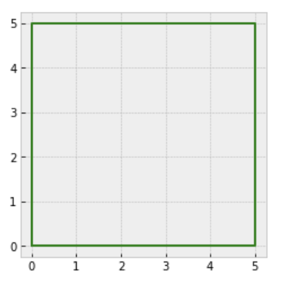
Problem 13-2
Location: assignment-problems/detecting_biased_coins.py
Grading: 4 points
Suppose that you run an experiment where you flip a coin 3 times, and repeat that trial 25 times. You run this experiment on 3 different coins, and get the following results:
coin_1 = ['TTH', 'HHT', 'HTH', 'TTH', 'HTH',
'TTH', 'TTH', 'TTH', 'THT', 'TTH',
'HTH', 'HTH', 'TTT', 'HTH', 'HTH',
'TTH', 'HTH', 'TTT', 'TTT', 'TTT',
'HTT', 'THT', 'HHT', 'HTH', 'TTH']
coin_2 = ['HTH', 'HTH', 'HTT', 'THH', 'HHH',
'THH', 'HHH', 'HHH', 'HTT', 'TTH',
'TTH', 'HHT', 'TTH', 'HTH', 'HHT',
'THT', 'THH', 'THT', 'TTH', 'TTT',
'HHT', 'THH', 'THT', 'THT', 'TTT']
coin_3 = ['HHH', 'THT', 'HHT', 'HHT', 'HTH',
'HHT', 'HHT', 'HHH', 'TTT', 'THH',
'HHH', 'HHH', 'TTH', 'THH', 'THH',
'TTH', 'HTT', 'TTH', 'HTT', 'HHT',
'TTH', 'HTH', 'THT', 'THT', 'HTH']Let $P_i(x)$ be the experimental probability of getting $x$ heads in a trial of 3 tosses, using the $i$th coin. Plot the distributions $P_1(x),$ $P_2(x),$ and $P_3(x)$ on the same graph. Be sure to label them.
- (This is similar to when you plotted the Monte Carlo distributions, but this time you're given the simulation results.)
Based on the plot of the distributions, what conclusions can you make about the coins? For each coin, does it appear to be fair, biased towards heads, or biased towards tails? Write your answer as a comment.
Problem 12-1
Location: assignment-problems/tally_sort.py
Grading: 4 points
Write a function tally_sort(num_list) that sorts the list num_list from least to greatest using the following process:
Subtract the minimum from the list so that the minimum is now 0.
Create an array whose indices correspond to the numbers from 0 to the maximum element.
Go through the list
num_listand tally up the count for each index.Transform the tallies into the desired sorted list (with the minimum still equal to 0).
Add the minimum back to get the desired sorted list, with the minimum now equal to the original minimum.
For example, if x = [2, 5, 2, 3, 8, 6, 3], then the process would be as follows:
identify the minimum: 2
subtract off the minimum: [0, 3, 0, 1, 6, 4, 1]
array of tallies: [number of instances of 0, number of instances of 1, number of instances of 2, number of instances of 3, number of instances of 4, number of instances of 5, number of instances of 6]
array of tallies: [0, 0, 0, 0, 0, 0, 0]
loop through the list [0, 3, 0, 1, 6, 4, 1]
first element: 0
increment the array of tallies at index 0
array of tallies: [1, 0, 0, 0, 0, 0, 0]
next element: 3
increment the array of tallies at index 3
array of tallies: [1, 0, 0, 1, 0, 0, 0]
next element: 0
increment the array of tallies at index 0
array of tallies: [2, 0, 0, 1, 0, 0, 0]
next element: 1
increment the array of tallies at index 1
array of tallies: [2, 1, 0, 1, 0, 0, 0]
next element: 6
increment the array of tallies at index 6
array of tallies: [2, 1, 0, 1, 0, 0, 1]
next element: 4
increment the array of tallies at index 4
array of tallies: [2, 1, 0, 1, 1, 0, 1]
next element: 1
increment the array of tallies at index 1
array of tallies: [2, 2, 0, 1, 1, 0, 1]
final array of tallies: [2, 2, 0, 1, 1, 0, 1]
remember what array of tallies represents: [number of instances of 0, number of instances of 1, number of instances of 2, number of instances of 3, number of instances of 4, number of instances of 5, number of instances of 6]
2 instances of 0 --> 0, 0
2 instances of 1 --> 1, 1
0 instances of 2 -->
1 instances of 3 --> 3
1 instances of 4 --> 4
0 instances of 5 -->
1 instances of 6 --> 6
Transform the tallies into the sorted list (with minimum still equal to 0)
[0, 0, 1, 1, 3, 4, 6]
Add the minimum back: [2, 2, 3, 3, 5, 6, 8]Assert that your function passes the following test:
>>> tally_sort([2, 5, 2, 3, 8, 6, 3])
[2, 2, 3, 3, 5, 6, 8]Note: Don't use the built-in functions max() nor min(). Rather, if you want to use either of these functions, you should write your own.
Problem 12-2
Location: assignment-problems/shapes.py
Grading: 4 points total
Observe the following plotting example:
import matplotlib.pyplot as plt
plt.style.use('bmh')
plt.plot(
[0, 1, 2, 0], # X-values
[0, 1, 0, 0], # Y-values
color='blue'
)
plt.gca().set_aspect("equal")
plt.savefig('triangle.png')

a. (2 points)
Write a class Rectangle.
include the attributes
base,height,color,perimeter,area, andvertices.- only
base,height, andcolorshould be used as parameters
- only
include a method
describe()that prints out the attributes of the rectangle.include a method
render()that renders the rectangle on a cartesian plane. (You can useplt.plot()andplt.gca()andplot.gca().set_aspect("equal")as shown above.)
>>> rect = Rectangle(5,2,'red')
>>> rect.describe()
Base: 5
Height: 2
Color: red
Perimeter: 14
Area: 10
Vertices: [(0,0), (5,0), (5,2), (0,2)]
>>> rect.render()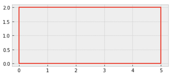
b. (2 points)
Write a class RightTriangle.
Include the attributes
base,height,color,perimeter,area, andvertices.Include a method
describe()that prints out the attributes of the right triangle.include a method
render()that draws the triangle on a cartesian plane.
>>> tri = RightTriangle(5,2,'blue')
>>> tri.describe()
Base: 5
Height: 2
Color: blue
Perimeter: 12.3851648071
Area: 5
Vertices: [(0,0), (5,0), (0,2)]
>>> tri.render()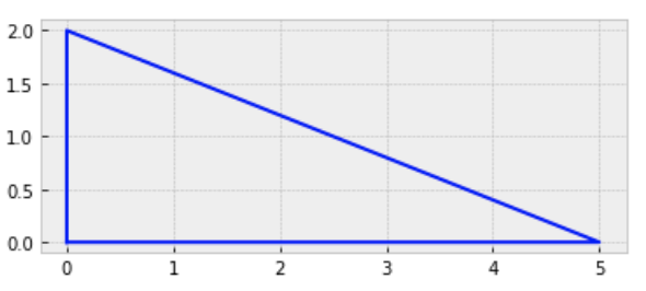
Problem 11-1
Location: assignment-problems/kl_divergence_for_monte_carlo_simulations.py
Grading: 10 points total
The Kullback–Leibler divergence (or relative entropy) between two probability distributions $p(n)$ and $q(n)$ is defined as
\begin{align*} \mathcal{D}(p \, || \, q) = \sum\limits_{n \text{ such that} \\ p(n), q(n) \neq 0} p(n) \ln \left( \dfrac{p(n)}{q(n)} \right) \end{align*}Intuitively, the divergence measures how "different" the two distributions are.
a. (4 points)
Write a function kl_divergence(p, q) that computes the KL divergence between two probability distributions p and q, represented as arrays. Test your function by asserting that it passes the following test:
>>> p = [0.2, 0.5, 0, 0.3]
>>> q = [0.1, 0.8, 0.1, 0]
>>> kl_divergence(p,q)
-0.09637237851 (in your test, you can round to 6 decimal places)
Note: the computation for the above is
0.2*ln(0.2/0.1) + 0.5*ln(0.5/0.8)
we exclude the terms 0*ln(0/0.1) and 0.3*ln(0.3/0)
because we're only summing over terms where neither
p(n) nor q(n) is equal to 0b. (4 points)
Compute the KL divergence where p is the Monte Carlo distribution and q is the true distribution for the number of heads in 8 coin tosses, using 1,000 samples in your Monte Carlo simulation (that's the default number from the previous assignment).
Then do the same computation with 100 samples, and then with 10,000 samples. Print out the results for all 3 computations:
>>> python assignment-problems/kl_divergence_for_monte_carlo_simulations.py
Testing KL Divergence... Passed!
Computing KL Divergence for MC Simulations...
100 samples --> KL Divergence = ___
1,000 samples --> KL Divergence = ___
10,000 samples --> KL Divergence = ___c. (2 points)
In a comment in your code, write down what the general trend is and why:
# As the number of samples increases, the KL divergence approaches __________ because _______________________________.Problem 11-2
Locations:
machine-learning/src/matrix.py
machine-learning/tests/test_matrix.py
Grading: 5 points for each passing test, 10 points code quality (so 20 points total)
MINOR CODE UPDATES BEFORE YOU DO THE ACTUAL PROBLEM:
Before you do this problem, you need to update some of your previous code so that you don't run into any mutation issues where running methods affects the underlying elements.
a. First, update your `copy()` method so that when it creates a copied matrix, it uses a completely separate array of elements (albeit with the same entries). You can do it like this:
def copy(self):
copied_elements = [[entry for entry in row] for row in self.elements]
return Matrix(copied_elements)(The reason why we need to do this is that whenever Python sees any sort of assignment with an existing list, it doesn't actually make a separate copy of the list. It just "points" to the existing list. We want the copied elements to be completely separate from self.elements.)
b. Second, update your helper methods `self.swap_rows()`, `self.normalize_row()`, `self.clear_below()`, and `self.clear_above()` so that they don't affect the original matrix `self`. In these methods, instead of modifying self.elements you should create a copy of self.elements, modify the copy, and then return the matrix whose elements are the copy.
You will need to update your tests to use A = A.swap_rows(), A = A.normalize_row(), A = A.clear_below(), and A = A.clear_above() as follows:
>>> A = Matrix(elements = [[0, 1, 2],
[3, 6, 9],
[2, 6, 8]])
>>> A.get_pivot_row(0)
1
>>> A = A.swap_rows(0,1)
>>> A.elements
[[3, 6, 9]
[0, 1, 2]
[2, 6, 8]]
>>> A = A.normalize_row(0)
>>> A.elements
[[1, 2, 3]
[0, 1, 2]
[2, 6, 8]]
>>> A = A.clear_below(0)
>>> A.elements
[[1, 2, 3]
[0, 1, 2]
[0, 2, 2]]
>>> A = A.get_pivot_row(1)
1
>>> A = A.normalize_row(1)
>>> A.elements
[[1, 2, 3]
[0, 1, 2]
[0, 2, 2]]
>>> A = A.clear_below(1)
>>> A.elements
[[1, 2, 3]
[0, 1, 2]
[0, 0, -2]]
>>> A.get_pivot_row(2)
2
>>> A = A.normalize_row(2)
>>> A.elements
[[1, 2, 3]
[0, 1, 2]
[0, 0, 1]]
>>> A = A.clear_above(2)
>>> A.elements
[[1, 2, 0]
[0, 1, 0]
[0, 0, 1]]
>>> A = A.clear_above(1)
>>> A.elements
[[1, 0, 0]
[0, 1, 0]
[0, 0, 1]]THE ACTUAL PROBLEM:
Extend your Matrix class to include a method rref that converts the matrix to reduced row echelon form. You should use the row reduction algorithm, which goes like this:
create a copy of the original matrix
row_index = 0
for each col_index:
if a pivot row exists for the col_index:
if the pivot row is not the current row:
swap the current row with the pivot row
# now the current row is actually the pivot row
normalize the pivot row so that the first nonzero entry is 1
clear all entries below and above the pivot entry
row_index += 1Assert that your method passes the following tests:
>>> A = Matrix([[0, 1, 2],
[3, 6, 9],
[2, 6, 8]])
>>> A.rref().elements
[1, 0, 0]
[0, 1, 0]
[0, 0, 1]
>>> B = Matrix([[0, 0, -4, 0],
[0, 0, 0.3, 0],
[0, 2, 1, 0]])
>>> A.rref().elements
[0, 1, 0, 0]
[0, 0, 1, 0]
[0, 0, 0, 0]To help you debug your implementation, here is a walkthrough of the above algorithm on the matrix $\begin{bmatrix} 0 & 1 & 2 \\ 3 & 6 & 9 \\ 2 & 6 & 8 \end{bmatrix}\mathbin{:}$
row_index = 0
looping through columns...
col_index = 0
current matrix is
[0,1,2]
[3,6,9]
[2,6,8]
for col_index = 0, the pivot row has index 1
this is different from row_index = 0, so we need to swap
swapping, the matrix becomes
[3,6,9]
[0,1,2]
[2,6,8]
the pivot row now has index 0, same as row_index = 0
normalizing the pivot row, the matrix becomes
[1,2,3]
[0,1,2]
[2,6,8]
the pivot entry is the 1 in the (0,0) position (i.e. top-left)
clearing all entries above and below the pivot entry, the matrix becomes
[1,2,3]
[0,1,2]
[0,2,2]
row_index += 1
so now we have row_index = 1
col_index = 1
current matrix is
[1,2,3]
[0,1,2]
[0,2,2]
for col_index = 1, the pivot row has index 1, same as row_index=1
so no swap is needed
the pivot row is already normalized
the pivot entry is the 1 in the (1,1) position (i.e. exact middle)
clearing all entries above and below the pivot entry, the matrix becomes
[1,0,-1]
[0,1,2]
[0,0,-2]
row_index += 1
so now we have row_index = 2
col_index = 2
current matrix is
[1,0,-1]
[0,1,2]
[0,0,-2]
for col_index = 2, the pivot row has index 2, same as row_index=2
so no swap is needed
normalizing the pivot row, the matrix becomes
[1,0,-1]
[0,1,2]
[0,0,1]
the pivot entry is the 1 in the (2,2) position (i.e. bottom-right)
clearing all entries above and below the pivot entry, the matrix becomes
[1,0,0]
[0,1,0]
[0,0,1]
row_index += 1
so now we have row_index = 3
we've gone through all the columns, so we're done!
the result is
[1,0,0]
[0,1,0]
[0,0,1]Likewise, here is a walkthrough of the above algorithm on the matrix $\begin{bmatrix} 0 & 0 & -4 & 0 \\ 0 & 0 & 0.3 & 0 \\ 0 & 2 & 1 & 0 \end{bmatrix}\mathbin{:}$
row_index = 0
looping through columns...
col_index = 0
current matrix is
[0,0,-4,0]
[0,0,0.3,0]
[0,2,1,0]
for col_index = 0, there is no pivot row
so we move on
we still have row_index = 0
col_index = 1
current matrix is
[0,0,-4,0]
[0,0,0.3,0]
[0,2,1,0]
for col_index = 1, the pivot row has index 2
this is different from row_index = 0, so we need to swap
swapping, the matrix becomes
[0,2,1,0]
[0,0,0.3,0]
[0,0,-4,0]
the pivot row now has index 0, same as row_index = 0
normalizing the pivot row, the matrix becomes
[0,1,0.5,0]
[0,0,0.3,0]
[0,0,-4,0]
the pivot entry is the 1 in the (0,1) position
all entries above and the pivot entry are already cleared
row_index += 1
so now we have row_index = 1
col_index = 2
current matrix is
[0,1,0.5,0]
[0,0,0.3,0]
[0,0,-4,0]
for col_index = 2, the pivot row has index 1, same as row_index = 1
so no swap is needed
normalizing the pivot row, the matrix becomes
[0,1,0.5,0]
[0,0,1,0]
[0,0,-4,0]
the pivot entry is the 1 in the (1,2) position
clearing all entries above and below the pivot entry, the matrix becomes
[0,1,0,0]
[0,0,1,0]
[0,0,0,0]
row_index += 1
so now we have row_index = 2
col_index = 3
current matrix is
[0,1,0,0]
[0,0,1,0]
[0,0,0,0]
for col_index = 3, there is no pivot row
so we move on
we still have row_index = 2
we've gone through all the columns, so we're done!
the result is
[0,1,0,0]
[0,0,1,0]
[0,0,0,0]Problem 10-1
Location: assignment-problems/distribution_plots.py
Grading: 6 points
Using your function probability(num_heads, num_flips), plot the distribution for the number of heads in 8 coin flips. In other words, plot the curve $y=p(x),$ where $p(x)$ is the probability of getting $x$ heads in $8$ coin flips.
Then, make 5 more plots, each using your function monte_carlo_probability(num_heads, num_flips). Put all your plots on the same graph, label them with a legend to indicate whether each plot is the true distribution or a monte carlo simulation, and save the figure as plot.png.
Legend: True, MC 1, MC 2, MC 3, MC 4, MC 5.
Make the true distribution thick (linewidth=2.5) and the monte carlo distributions thin (linewidth=0.75). A plotting example for 4 coin flips is shown below to assist you.
Note: You will need to modify the plotting example to make it for 8 coin flips instead of 4.
To be clear, you are just making 1 plot. The plot should contain the true distribution (thick line) and 5 Monte Carlo simulation distributions (thin lines).
import matplotlib.pyplot as plt
plt.style.use('bmh')
plt.plot([0,1,2,3,4],[0.1, 0.3, 0.5, 0.1, 0.1],linewidth=2.5)
plt.plot([0,1,2,3,4],[0.3, 0.1, 0.4, 0.2, 0.1],linewidth=0.75)
plt.plot([0,1,2,3,4],[0.2, 0.2, 0.3, 0.3, 0.2],linewidth=0.75)
plt.legend(['True','MC 1','MC 2'])
plt.xlabel('Number of Heads')
plt.ylabel('Probability')
plt.title('True Distribution vs Monte Carlo Simulations for 4 Coin Flips')
plt.savefig('plot.png')

Problem 10-2
Locations: assignment-problems/unlist.py
Grading: In each part, you get 1 point for code quality, and 1 point for passing tests (so 4 points total)
a. WITHOUT using recursion, create a function unlist_nonrecursive(x) that removes outer parentheses from a list until either a) the final list consists of multiple elements, or b) no more lists exist.
Assert that your function passes the following tests.
>>> unlist_nonrecursive([[[[1], [2,3], 4]]])
[[1], [2,3], 4]
>>> unlist_nonrecursive([[[[1]]]])
1b. USING RECURSION, write a function unlist_recursive(x) and assert that it passes the same tests as in part (a).
Problem 9-1
Locations: assignment-problems/collatz_iterations.py
The Collatz function is defined as
$$f(n) = \begin{cases} n \, / \, 2 & \text{if } n \text{ is even} \\ 3n+1 & \text{if } n \text{ is odd} \end{cases}$$The Collatz conjecture is that by repeatedly applying this function to any positive number, the result will eventually reach the cycle
$$1 \to 4 \to 2 \to 1.$$For example, repeatedly applying the Collatz function to the number $13,$ we have:
$$13 \to 40 \to 20 \to 10 \to 5 \to 16 \to 8 \to 4 \to 2 \to 1$$a. (1 point for code quality; 1 point for passing the test)
Create a function collatz_iterations(number) that computes the number of iterations of the Collatz function that it takes for the input number to reach $1.$
>>> collatz_iterations(13)
9b. (1 point)
Write a short script to answer the following question:
Of the numbers from 1 to 1000, which number has the highest number of Collatz iterations?
c. (1 point)
Make a plot where the horizontal axis is the numbers from 1 to 1000 and the vertical axis is the number of Collatz iterations. You can use the sample code below to help you with plotting.
import matplotlib.pyplot as plt
plt.style.use('bmh')
x_coords = [0,1,2,3,4]
y_coords = [5,3,8,5,1]
plt.plot(x_coords, y_coords)
plt.xlabel('X-Axis Label')
plt.ylabel('Y-Axis Label')
plt.title('This is the title of the plot!')
plt.savefig('plot.png')

Problem 9-2
This will be a lighter assignment in case you need to catch up with the Matrix class or the Monte Carlo simulations. They need to be working 100%. Make sure that you've caught up, because we will be pressing forward with them on the next few assignments.
Problem 8-1
Locations: machine-learning/src/matrix.py and machine-learning/tests/test_matrix.py
Grading: 5 points for code quality; 5.5 points for passing tests (0.5 point per test)
Implement the following helper methods in your matrix class.
get_pivot_row(self, column_index): returns the index of the topmost row that has a nonzero entry in the desiredcolumn_indexand such that all entries left ofcolumn_indexare zero. Otherwise, if no row exists, returnNone.swap_rows(self, row_index1, row_index2): swap the row atrow_index1with the row atrow_index2.normalize_row(self, row_index): divide the entire row atrow_indexby the row's first nonzero entry.clear_below(self, row_index):- Let $j$ be the column index of the first nonzero entry in the row at
row_index. - Subtract multiples of the row at
row_indexfrom the rows below, so that for any row belowrow_index, the entry at column $j$ is zero.
- Let $j$ be the column index of the first nonzero entry in the row at
clear_above(self, row_index):- Let $j$ be the column index of the first nonzero entry in the row at
row_index. - Subtract multiples of the row at
row_indexfrom the rows above, so that for any row aboverow_index, the entry at column $j$ is zero.
- Let $j$ be the column index of the first nonzero entry in the row at
Watch out!
Remember that the first row/column of a matrix has the index
0, not1.If
row1is "below"row2in a matrix, thenrow1actually has a higher index thanrow2. This is because the0index corresponds to the very top row.
Assert that the following tests pass.
>>> A = Matrix(elements = [[0, 1, 2],
[3, 6, 9],
[2, 6, 8]])
>>> A.get_pivot_row(0)
1
>>> A = A.swap_rows(0,1)
>>> A.elements
[[3, 6, 9]
[0, 1, 2]
[2, 6, 8]]
>>> A = A.normalize_row(0)
>>> A.elements
[[1, 2, 3]
[0, 1, 2]
[2, 6, 8]]
>>> A = A.clear_below(0)
>>> A.elements
[[1, 2, 3]
[0, 1, 2]
[0, 2, 2]]
>>> A = A.get_pivot_row(1)
1
>>> A = A.normalize_row(1)
>>> A.elements
[[1, 2, 3]
[0, 1, 2]
[0, 2, 2]]
>>> A = A.clear_below(1)
>>> A.elements
[[1, 2, 3]
[0, 1, 2]
[0, 0, -2]]
>>> A.get_pivot_row(2)
2
>>> A = A.normalize_row(2)
>>> A.elements
[[1, 2, 3]
[0, 1, 2]
[0, 0, 1]]
>>> A = A.clear_above(2)
>>> A.elements
[[1, 2, 0]
[0, 1, 0]
[0, 0, 1]]
>>> A = A.clear_above(1)
>>> A.elements
[[1, 0, 0]
[0, 1, 0]
[0, 0, 1]]Make sure that when you run python tests/test_matrix.py, your tests print out (including your tests from last time)
>>> python tests/test_matrix.py
Testing method "copy"...
PASSED
Testing method "add"...
PASSED
Testing method "subtract"...
PASSED
Testing method "scalar_multiply"...
PASSED
Testing method "matrix_multiply"...
PASSED
Testing row reduction on the following matrix:
[[0, 1, 2],
[3, 6, 9],
[2, 6, 8]]
- Testing method "get_pivot_row(0)"...
- PASSED
- Testing method "swap_rows(0,1)"...
- PASSED
- Testing method "normalize_row(0)"...
- PASSED
- Testing method "clear_below(0)"...
- PASSED
- Testing method "get_pivot_row(1)"...
- PASSED
- Testing method "normalize_row(1)"...
- PASSED
- Testing method "clear_below(1)"...
- PASSED
- Testing method "get_pivot_row(2)"...
- PASSED
- Testing method "normalize_row(2)"...
- PASSED
- Testing method "clear_above(2)"...
- PASSED
- Testing method "clear_above(1)"...
- PASSEDProblem 8-2
Locations: assignment-problems/further_comprehensions.py
Grading: 2 points for each part
a. USING COMPREHENSION, create a function identity_matrix_elements(n) that creates the elements for an $n \times n$ identity matrix. The body of your function should consist of just 1 line, in which it simply returns a list comprehension.
Assert that your function passes the following test:
>>> identity_matrix_elements(4)
[[1, 0, 0, 0],
[0, 1, 0, 0],
[0, 0, 1, 0],
[0, 0, 0, 1]]- Hint:
[[(some expression) for each column index] for each row index]
b. USING COMPREHENSION, create a function counting_across_rows_matrix_elements(m,n) that creates the elements for an $m \times n$ matrix that "counts" upwards across the rows. The body of your function should consist of just 1 line, in which it simply returns a list comprehension.
Assert that your function passes the following test:
>>> counting_across_rows_matrix_elements(3,4)
[[1, 2, 3, 4],
[5, 6, 7, 8],
[9, 10, 11, 12]]- Hint:
[[(some expression) for each column index] for each row index]
Note: Try to do these problems without without using any separate functions in the (some expression) part. But if you can't figure it out, you can define an outside function to use there, and I won't take off points.
Problem 7-1
Grading: 1 point per working test with good code quality. (There are 7 tests total)
Generalize your Matrix class to $M \times N$ matrices. Also, write two more methods transpose() and is_equal(), and create attributes num_rows and num_cols.
Assert that the following tests work. Put your tests in machine-learning/tests/test_matrix.py.
Note: In the tests below, we manipulate a $4 \times 5$ matrix. However, your code should be general to any size of matrix. For example, it should work with a $400 \times 500$ matrix as well.
>>> A = Matrix([[1,0,2,0,3],
[0,4,0,5,0],
[6,0,7,0,8],
[-1,-2,-3,-4,-5])
>>> (A.num_rows, A.num_cols)
(4, 5)
>>> A_t = A.transpose()
>>> A_t.elements
[[ 1, 0, 6, -1],
[ 0, 4, 0, -2],
[ 2, 0, 7, -3],
[ 0, 5, 0, -4],
[ 3, 0, 8, -5]]
>>> B = A_t.matrix_multiply(A)
>>> B.elements
[[38, 2, 47, 4, 56],
[ 2, 20, 6, 28, 10],
[47, 6, 62, 12, 77],
[ 4, 28, 12, 41, 20],
[56, 10, 77, 20, 98]]
>>> C = B.scalar_multiply(0.1)
>>> C.elements
[[3.8, .2, 4.7, .4, 5.6],
[ .2, 2.0, .6, 2.8, 1.0],
[4.7, .6, 6.2, 1.2, 7.7],
[ .4, 2.8, 1.2, 4.1, 2.0],
[5.6, 1.0, 7.7, 2.0, 9.8]]
>>> D = B.subtract(C)
>>> D.elements
[[34.2, 1.8, 42.3, 3.6, 50.4]
[ 1.8, 18. , 5.4, 25.2, 9. ]
[42.3, 5.4, 55.8, 10.8, 69.3]
[ 3.6, 25.2, 10.8, 36.9, 18. ]
[50.4, 9. , 69.3, 18. , 88.2]]
>>> E = D.add(C)
[[38, 2, 47, 4, 56],
[ 2, 20, 6, 28, 10],
[47, 6, 62, 12, 77],
[ 4, 28, 12, 41, 20],
[56, 10, 77, 20, 98]]
>>> (E.is_equal(B), E.is_equal(C))
(True, False)Tip: For matrix_multiply, make a helper function dot_product that computes a dot product of two lists. Then just loop through each row-column pair and compute the corresponding dot product.
Note: When you multiply 38 by 0.1, you might get a result like 3.80000000...3.
This is because of the way that Python represents numbers -- decimal numbers are always close approximations to the real thing, since there's a limit to how many digits the computer can store. So, it's normal.
However, that does make it more difficult to write a test to make sure that a matrix equals the desired result. So what you can do to get around it is you can implement a round method for your matrix, and then assert that your matrix elements (rounded to, say, 5 decimal places) come out to the desired result.
class Matrix
...
def round(self, num_decimal_places):
return self.elements rounded to num_decimal_placesscalar_product_matrix = original_matrix.scalar_multiply(0.1)
assert scalar_product_matrix.round(5) == desired_resultThat way, the 3.80000000...3 will get rounded to 38.00000, and 38.00000 == 38 will come out true.
For rounding, there's a built-in function round(). For example,
>>> round(0.45982345, 4)
0.4598Problem 7-2
Location: assignment-problems/monte_carlo_coin_flips.py
Grading: There are 6 points possible (2 points per part).
In this problem, you will compute the probability of getting num_heads heads in num_flips flips of a fair coin. You will do this using two different methods. You should write your functions in a file assignment-problems/coin_flipping.py
a. (1 point for code quality; 1 point for passing test)
Write a function probability(num_heads, num_flips) that uses mathematics to compute the probability.
First, compute the total number of possible outcomes for
num_flipsflips. (Hint: it's an exponent.)Then, compute the number of outcomes in which
num_headsheads arise innum_flipsflips. (Hint: it's a combination.)Then, divide the results.
For a
factorialfunction and or abinomial_coefficientfunction, write your own from scratch.
Assert that your function passes the following test:
>>> probability(5,8)
0.21875b. (2 points for code quality/correctness)
Write a function monte_carlo_probability(num_heads, num_flips) that uses simulation to compute the probability.
First, simulate 1000 trials of
num_flipscoin flips, keeping track of how many heads there were.Then, divide the number of outcomes in which there were
num_headsheads, by the total number of trials (1000).You can use the
random()function from therandomlibrary:>>> from random import random >>> random() (some random number between 0 and 1)
c. (1 point for code quality; 1 point for printing out reasonable monte carlo results)
When you run assignment-problems/monte_carlo_coin_flips.py, you should print out the result of probability(5,8). Also, print out 5 instances of monte_carlo_probability(5,8).
- The 5 instances will be slightly different because it's a random simulation, but they should be fairly close to each other and to the true result.
Problem 7-3
Location: assignment-problems/swap_sort_theory.txt
Grading: 1 point per correct answer with justification.
Answer the following questions about swap_sort. Explain or show your work for each question.
a. Given a list of 5 elements, what’s the least number of swaps that could occur? What about for a list of $n$ elements? Explain why.
b. Given a list of 5 elements, what’s the greatest number of swaps that could occur? What about for a list of $n$ elements? Explain why.
For (c) and (d), determine whether the statement is true or false. If true, then explain why. If false, then provide a counterexample.
c. The number of swaps performed by swap sort on each pass is always a decreasing sequence.
d. On two consecutive passes, the number of swaps performed by swap sort is never equal.
Problem 6-1
Locations: machine-learning/src/matrix.py and machine-learning/tests/test_matrix.py
Grading: 5 points for code quality; 5 points for passing each test (1 point per test)
Note: You are NOT allowed to use numpy or any other external library. The Matrix class should be written entirely from scratch.
Create a
machine-learningrepository on GitHub and connect it to a repl of the same name. Create a foldermachine-learning/src, and within that folder, put a filematrix.pywhich will contain theMatrixclass you write in this problem.In
machine-learning/src/matrix.py, create aMatrixclass with the methodscopy,add, andsubtract,scalar_multiply, andmatrix_multiplyfor $2 \times 2$ matrices.Create a folder
machine-learning/tests, and within that folder, put a filetest_matrix.pywhich will contain your "assert" tests for theMatrixclass.In
machine-learning/tests/test_matrix.py, include the following at the top of your file so that you can use yourMatrixclass:
import sys
sys.path.append('src')
from matrix import Matrix- In
machine-learning/tests/test_matrix.py, assert that yourMatrixclass passes the following tests:
>>> A = Matrix([[1,3],
[2,4]])
>>> A.elements
[[1,3],
[2,4]]
>>> B = A.copy()
>>> A = 'resetting A to a string'
>>> B.elements # the purpose of this test is to show that B is independent of A
[[1,3],
[2,4]]
>>> C = Matrix([[1,0],
[2,-1]])
>>> D = B.add(C)
>>> D.elements
[[2,3],
[4,3]]
>>> E = B.subtract(C)
>>> E.elements
[[0,3],
[0,5]]
>>> F = B.scalar_multiply(2)
>>> F.elements
[[2,6],
[4,8]]
>>> G = B.matrix_multiply(C)
[[7,-3],
[10,-4]]- Make sure that when you run
python tests/test_matrix.py, your tests print out:
>>> python tests/test_matrix.py
Testing method "copy"...
PASSED
Testing method "add"...
PASSED
Testing method "subtract"...
PASSED
Testing method "scalar_multiply"...
PASSED
Testing method "matrix_multiply"...
PASSEDProblem 6-2
Locations: assignment-problems/skip_factorial.py
Grading: For each part, you get 1 point for code quality and 1 point for passing both tests.
a. WITHOUT using recursion, create a function skip_factorial_nonrecursive(n) that computes the product
- $n(n-2)(n-4)\ldots(2)$ if $n$ is even, or
- $n(n-2)(n-4)\ldots(1)$ if $n$ is odd.
Assert that your function passes the following tests:
>>> skip_factorial_nonrecursive(6)
48
>>> skip_factorial_nonrecursive(7)
105b. USING RECURSION, create a function skip_factorial_recursive(n) and assert that it passes the same tests as in part (a).
Problem 6-3
Locations: assignment-problems/simple_sort_swap_sort.py
Note: In these questions, you will need to compute the minimum element of a list without using Python's built-in min function. To do this, you should write a "helper" function minimum() that loops through a list, keeping track of the smallest element seen so far. For example:
given the list [4,6,3,5]
first element is 4; smallest element so far is 4
next element is 6; smallest element so far is 4
next element is 3; smallest element so far is 3
next element is 5; smallest element so far is 3
conclude that minimum element is 3a. (1 point for code quality, 1 point for passing test)
Write a function simple_sort(num_list) that takes an input list num_list and sorts its elements from least to greatest by repeatedly finding the smallest element and moving it to a new list. Don't use Python's built-in min function or its built-in sort function.
Assert that your function passes the following test:
>>> simple_sort([5,8,2,2,4,3,0,2,-5,3.14,2])
[-5,0,2,2,2,2,3,3.14,4,5,8]Tip: To help you debug your code, here are the steps that your function should be doing behind the scenes. (You don't have to write tests for them.)
sorted elements: []
remaining elements: [5,8,2,2,4,3,0,2,-5,3.14,2]
minimum of remaining elements: -5
sorted elements: [-5]
remaining elements: [5,8,2,2,4,3,0,2,3.14,2]
minimum of remaining elements: 0
sorted elements: [-5,0]
remaining elements: [5,8,2,2,4,3,2,3.14,2]
minimum of remaining elements: 2
sorted elements: [-5,0,2]
remaining elements: [5,8,2,4,3,2,3.14,2]
minimum of remaining elements: 2
sorted elements: [-5,0,2,2]
remaining elements: [5,8,4,3,2,3.14,2]
minimum of remaining elements: 2
sorted elements: [-5,0,2,2,2]
remaining elements: [5,8,4,3,3.14,2]
minimum of remaining elements: 2
sorted elements: [-5,0,2,2,2,2]
remaining elements: [5,8,4,3,3.14]
minimum of remaining elements: 3
sorted elements: [-5,0,2,2,2,2]
remaining elements: [5,8,4,3.14]
minimum of remaining elements: 3.14
sorted elements: [-5,0,2,2,2,2,3.14]
remaining elements: [5,8,4]
minimum of remaining elements: 4
sorted elements: [-5,0,2,2,2,2,3.14,4]
remaining elements: [5,8]
minimum of remaining elements: 5
sorted elements: [-5,0,2,2,2,2,3.14,4,5]
remaining elements: [8]
minimum of remaining elements: 8
sorted elements: [-5,0,2,2,2,2,3.14,4,5,8]
remaining elements: []
final output: [-5,0,2,2,2,2,3.14,4,5,8]b. (1 point for code quality, 1 point for passing test)
Write a function swap_sort(x) that sorts the list from least to greatest by repeatedly going through each pair of adjacent elements and swapping them if they are in the wrong order. The algorithm should terminate once it's made a full pass through the list without making any more swaps. Don't use Python's built-in sort function.
Assert that your function passes the following test:
>>> swap_sort([5,8,2,2,4,3,0,2,-5,3.14,2])
[-5,0,2,2,2,2,3,3.14,4,5,8]Tip: To help you debug your code, here are the steps that your function should be doing behind the scenes. (You don't have to write tests for them.)
FIRST PASS
starting list: [-5,0,2,2,2,2,3,3.14,4,5,8]
[(5,8),2,2,4,3,0,2,-5,3.14,2]
[5,(8,2),2,4,3,0,2,-5,3.14,2] SWAP
[5,2,(8,2),4,3,0,2,-5,3.14,2] SWAP
[5,2,2,(8,4),3,0,2,-5,3.14,2] SWAP
[5,2,2,4,(8,3),0,2,-5,3.14,2] SWAP
[5,2,2,4,3,(8,0),2,-5,3.14,2] SWAP
[5,2,2,4,3,0,(8,2),-5,3.14,2] SWAP
[5,2,2,4,3,0,2,(8,-5),3.14,2] SWAP
[5,2,2,4,3,0,2,-5,(8,3.14),2] SWAP
[5,2,2,4,3,0,2,-5,3.14,(8,2)] SWAP
ending list: [5,2,2,4,3,0,2,-5,3.14,2,8]
SECOND PASS
starting list: [5,2,2,4,3,0,2,-5,3.14,2,8]
[(5,2),2,4,3,0,2,-5,3.14,2,8] SWAP
[2,(5,2),4,3,0,2,-5,3.14,2,8] SWAP
[2,2,(5,4),3,0,2,-5,3.14,2,8] SWAP
[2,2,4,(5,3),0,2,-5,3.14,2,8] SWAP
[2,2,4,3,(5,0),2,-5,3.14,2,8] SWAP
[2,2,4,3,0,(5,2),-5,3.14,2,8] SWAP
[2,2,4,3,0,2,(5,-5),3.14,2,8] SWAP
[2,2,4,3,0,2,-5,(5,3.14),2,8] SWAP
[2,2,4,3,0,2,-5,3.14,(5,2),8] SWAP
[2,2,4,3,0,2,-5,3.14,2,(5,8)]
ending list: [2,2,4,3,0,2,-5,3.14,2,5,8]
THIRD PASS
starting list: [2,2,4,3,0,2,-5,3.14,2,5,8]
[(2,2),4,3,0,2,-5,3.14,2,5,8]
[2,(2,4),3,0,2,-5,3.14,2,5,8]
[2,2,(4,3),0,2,-5,3.14,2,5,8] SWAP
[2,2,3,(4,0),2,-5,3.14,2,5,8] SWAP
[2,2,3,0,(4,2),-5,3.14,2,5,8] SWAP
[2,2,3,0,2,(4,-5),3.14,2,5,8] SWAP
[2,2,3,0,2,-5,(4,3.14),2,5,8] SWAP
[2,2,3,0,2,-5,3.14,(4,2),5,8] SWAP
[2,2,3,0,2,-5,3.14,2,(4,5),8]
[2,2,3,0,2,-5,3.14,2,4,(5,8)]
ending list: [2,2,3,0,2,-5,3.14,2,4,5,8]
FOURTH PASS
starting list: [2,2,3,0,2,-5,3.14,2,4,5,8]
[(2,2),3,0,2,-5,3.14,2,4,5,8]
[2,(2,3),0,2,-5,3.14,2,4,5,8]
[2,2,(3,0),2,-5,3.14,2,4,5,8] SWAP
[2,2,0,(3,2),-5,3.14,2,4,5,8] SWAP
[2,2,0,2,(3,-5),3.14,2,4,5,8] SWAP
[2,2,0,2,-5,(3,3.14),2,4,5,8]
[2,2,0,2,-5,3,(3.14,2),4,5,8] SWAP
[2,2,0,2,-5,3,2,(3.14,4),5,8]
[2,2,0,2,-5,3,2,3.14,(4,5),8]
[2,2,0,2,-5,3,2,3.14,4,(5,8)]
ending list: [2,2,0,2,-5,3,2,3.14,4,5,8]
FIFTH PASS
starting list: [2,2,0,2,-5,3,2,3.14,4,5,8]
[(2,2),0,2,-5,3,2,3.14,4,5,8]
[2,(2,0),2,-5,3,2,3.14,4,5,8] SWAP
[2,0,(2,2),-5,3,2,3.14,4,5,8]
[2,0,2,(2,-5),3,2,3.14,4,5,8] SWAP
[2,0,2,-5,(2,3),2,3.14,4,5,8]
[2,0,2,-5,2,(3,2),3.14,4,5,8] SWAP
[2,0,2,-5,2,2,(3,3.14),4,5,8]
[2,0,2,-5,2,2,3,(3.14,4),5,8]
[2,0,2,-5,2,2,3,3.14,(4,5),8]
[2,0,2,-5,2,2,3,3.14,4,(5,8)]
ending list: [2,0,2,-5,2,2,3,3.14,4,5,8]
SIXTH PASS
starting list: [2,0,2,-5,2,2,3,3.14,4,5,8]
[(2,0),2,-5,2,2,3,3.14,4,5,8] SWAP
[0,(2,2),-5,2,2,3,3.14,4,5,8]
[0,2,(2,-5),2,2,3,3.14,4,5,8] SWAP
[0,2,-5,(2,2),2,3,3.14,4,5,8]
[0,2,-5,2,(2,2),3,3.14,4,5,8]
[0,2,-5,2,2,(2,3),3.14,4,5,8]
[0,2,-5,2,2,2,(3,3.14),4,5,8]
[0,2,-5,2,2,2,3,(3.14,4),5,8]
[0,2,-5,2,2,2,3,3.14,(4,5),8]
[0,2,-5,2,2,2,3,3.14,4,(5,8)]
ending list: [0,2,-5,2,2,2,3,3.14,4,5,8]
SEVENTH PASS
starting list: [0,2,-5,2,2,2,3,3.14,4,5,8]
[(0,2),-5,2,2,2,3,3.14,4,5,8]
[0,(2,-5),2,2,2,3,3.14,4,5,8] SWAP
[0,-5,(2,2),2,2,3,3.14,4,5,8]
[0,-5,2,(2,2),2,3,3.14,4,5,8]
[0,-5,2,2,(2,2),3,3.14,4,5,8]
[0,-5,2,2,2,(2,3),3.14,4,5,8]
[0,-5,2,2,2,2,(3,3.14),4,5,8]
[0,-5,2,2,2,2,3,(3.14,4),5,8]
[0,-5,2,2,2,2,3,3.14,(4,5),8]
[0,-5,2,2,2,2,3,3.14,4,(5,8)]
ending list: [0,-5,2,2,2,2,3,3.14,4,5,8]
EIGTHTH PASS
starting list: [0,-5,2,2,2,2,3,3.14,4,5,8]
[(0,-5),2,2,2,2,3,3.14,4,5,8] SWAP
[-5,(0,2),2,2,2,3,3.14,4,5,8]
[-5,0,(2,2),2,2,3,3.14,4,5,8]
[-5,0,2,(2,2),2,3,3.14,4,5,8]
[-5,0,2,2,(2,2),3,3.14,4,5,8]
[-5,0,2,2,2,(2,3),3.14,4,5,8]
[-5,0,2,2,2,2,(3,3.14),4,5,8]
[-5,0,2,2,2,2,3,(3.14,4),5,8]
[-5,0,2,2,2,2,3,3.14,(4,5),8]
[-5,0,2,2,2,2,3,3.14,4,(5,8)]
ending list: [-5,0,2,2,2,2,3,3.14,4,5,8]
NINTH PASS
starting list: [-5,0,2,2,2,2,3,3.14,4,5,8]
[(-5,0),2,2,2,2,3,3.14,4,5,8]
[-5,(0,2),2,2,2,3,3.14,4,5,8]
[-5,0,(2,2),2,2,3,3.14,4,5,8]
[-5,0,2,(2,2),2,3,3.14,4,5,8]
[-5,0,2,2,(2,2),3,3.14,4,5,8]
[-5,0,2,2,2,(2,3),3.14,4,5,8]
[-5,0,2,2,2,2,(3,3.14),4,5,8]
[-5,0,2,2,2,2,3,(3.14,4),5,8]
[-5,0,2,2,2,2,3,3.14,(4,5),8]
[-5,0,2,2,2,2,3,3.14,4,(5,8)]
ending list: [-5,0,2,2,2,2,3,3.14,4,5,8]
no swaps were done in the ninth pass, so we're done!
final output: [-5,0,2,2,2,2,3,3.14,4,5,8]Problem 5-1
Location: assignment-problems/comprehensions.py
Grading: 2 points for each part (a) and (b)
a. Implement a function even_odd_tuples that takes a list of numbers and labels each number as even or odd. Return a list comprehension so that the function takes up only two lines, as follows:
def even_odd_tuples(numbers):
return [<your code here>]Assert that your function passes the following test:
>>> even_odd_tuples([1,2,3,5,8,11])
[(1,'odd'),(2,'even'),(3,'odd'),(5,'odd'),(8,'even'),(11,'odd')]b. Implement a function even_odd_dict that again takes a list of numbers and labels each number as even or odd. This time, the output will be a dictionary. Use a dictionary comprehensions so that the function takes up only two lines, as follows:
def even_odd_dict(numbers):
return {<your code here>}Assert that your function passes the following test:
>>> even_odd_dict([1,2,3,5,8,11])
{
1:'odd',
2:'even',
3:'odd',
5:'odd',
8:'even',
11:'odd'
}Problem 5-2
Location: assignment-problems/root_approximation.py
Grading: For each part (a) and (b), you get 2 points for code quality and 2 points for passing the tests. So there are 8 points in total to be had on this problem.
The value of $\sqrt{2}$ is in the interval $[1,2].$ We will estimate the value of $\sqrt{2}$ by repeatedly narrowing these bounds.
a. Create a function update_bounds(bounds) that guesses a value halfway between the bounds, determines whether the guess was too high or too low, and updates the bounds accordingly.
For example, starting with the bounds $[1,2],$ the guess would be $1.5.$ This guess is too high because $1.5^2 = 2.25 > 2.$ So, the updated bounds would be $[1, 1.5].$
Now, using the bounds $[1,1.5]$, the next guess would be $1.25.$ This guess is too low because $1.25^2 = 1.5625 < 2.$ So, the updated bounds would be $[1.25, 1.5].$
Assert that your function passes the following tests:
>>> update_bounds([1, 2])
[1, 1.5]
>>> update_bounds([1, 1.5])
[1.25, 1.5]b. Write a function estimate_root(precision) that estimates the value of $\sqrt{2}$ by repeatedly calling update_bounds until the bounds are narrower than precision. You can start with the bounds $[1,2]$ again. Then it should return the midpoint of the final set of bounds.
Assert that your function passes the following test:
>>> estimate_root(0.1)
1.40625
note: the sequence of bounds would be
[1, 2]
[1, 1.5]
[1.25, 1.5]
[1.375, 1.5]
[1.375, 1.4375]Problem 5-3
Location: assignment-problems/queue.py
Grading: you get 0.5 points for passing each test, and 2 points for code quality
Implement a queue. That is, create a class Queue which operates on an attribute data using the following methods:
enqueue: add a new item to the back of the queuedequeue: remove the item at the front of the queuepeek: return the item at the front without modifying the queue
Assert that the following tests pass:
>>> q = Queue()
>>> q.data
[]
>>> q.enqueue('a')
>>> q.enqueue('b')
>>> q.enqueue('c')
>>> q.data
['a', 'b', 'c']
>>> q.dequeue()
>>> q.data
['b', 'c']
>>> q.peek()
'b'
>>> q.data
['b', 'c']Problem 4-1
Location: assignment-problems/flatten.py
Grading: 1 point for passing test, and then (assuming it passes the test) 1 point for code quality
Write a function flatten which takes a nested dictionary and converts it into a flat dictionary based on the key names. You can assume that the nested dictionary only has one level of nesting, meaning that in the output, each key will have exactly one underscore.
Assert that your function passes the following test:
>>> colors = {
'animal': {
'bumblebee': ['yellow', 'black'],
'elephant': ['gray'],
'fox': ['orange', 'white']
},
'food': {
'apple': ['red', 'green', 'yellow'],
'cheese': ['white', 'orange']
}
}
>>> flatten(colors)
{
'animal_bumblebee': ['yellow', 'black'],
'animal_elephant': ['gray'],
'animal_fox': ['orange', 'white'],
'food_apple': ['red', 'green', 'yellow'],
'food_cheese': ['white', 'orange']
}Problem 4-2
Location: assignment-problems/convert_to_base_2.py
Grading: 1 point for passing test, and then (assuming it passes the test) 1 point for code quality
Write a function convert_to_base_2 that converts a number from base-10 to base-2. Assert that it passes the following test:
>>> convert_to_base_2(19)
10011Hint: use $\log_2$ to figure out how many digits there will be in the binary number. Then, fill up the binary number, repeatedly subtracting off the next-largest power of 2 if possible.
Problem 4-3
Location: assignment-problems/linear_encoding_cryptography.py
Grading: for each part, you get 1 point for passing test, and then (assuming it passes the test) 1 point for code quality
In Assignment 1, we encountered the trivial encoding function which maps
' '$\rightarrow 0,$'a'$\rightarrow 1,$'b'$\rightarrow 2,$
and so on.
Using a linear encoding function $s(x) = 2x+3,$ the message 'a cat' can be encoded as follows:
Original message:
'a cat'Trivial encoding:
[1, 0, 3, 1, 20]Linear encoding:
[5, 3, 9, 5, 43]
a. Create a function encode(string,a,b) which encodes a string using the linear encoding function $s(x) = ax+b.$ Assert that your function passes the following test:
>>> get_encoding('a cat', 2, 3)
[5, 3, 9, 5, 43]b. Create a function decode(numbers,a,b) which attempts to decode a given list of numbers using the linear encoding function $s(x) = ax+b.$
To do this, you should apply the inverse encoding $s^{-1}(x) = \dfrac{x-b}{a},$ to all the numbers in the list and then check if they are all integers in the range from $0$ to $26$ (inclusive). If they are, then return the corresponding letters; if they are not, then return False.
Assert that your function passes the following tests:
>>> decode([5, 3, 9, 5, 43], 2, 3)
'a cat'
for debugging purposes, here's the scratch work for you:
[(5-3)/2, (3-3)/2, (9-3)/2, (5-3)/2, (43-3)/2]
[1, 0, 3, 1, 20]
'a cat'
>>> decode([1, 3, 9, 5, 43], 2, 3)
False
for debugging purposes, here's the scratch work for you:
[(1-3)/2, (3-3)/2, (9-3)/2, (5-3)/2, (43-3)/2]
[-1, 0, 3, 1, 20]
False (because -1 does not correspond to a letter)
>>> decode([5, 3, 9, 5, 44], 2, 3)
False
for debugging purposes, here's the scratch work for you:
[(5-3)/2, (3-3)/2, (9-3)/2, (5-3)/2, (44-3)/2]
[1, 0, 3, 1, 20.5]
False (because 20.5 does not correspond to a letter)c. Decode the message
[377,
717,
71,
513,
105,
921,
581,
547,
547,
105,
377,
717,
241,
71,
105,
547,
71,
377,
547,
717,
751,
683,
785,
513,
241,
547,
751],given that it was encoded with a linear encoding function $s(x) = ax+b$ where $a,b \in \{ 0, 1, 2, \ldots, 100 \}.$
You should run through each combination of $a$ and $b,$ try to decode the list of numbers using that combination, and if you get a valid decoding, then print it out. Then, you can visually inspect all the decodings you printed out to find the one that makes sense.
Problem 3-1
Location: assignment-problems/convert_to_base_10.py
Grading: 1 point for passing test, and then (assuming it passes the test) 1 point for code quality
Write a function convert_to_base_10 that converts a number from base-2 (binary) to base-10 (decimal). For example, the binary number $10011$ corresponds to the decimal number
$$
1 \cdot 2^{4} + 0 \cdot 2^3 + 0 \cdot 2^2 + 1 \cdot 2^1 + 1 \cdot 2^0 = 19.
$$
Assert that your function passes the following test:
>>> convert_to_base_10(10011)
19Problem 3-2
Location: assignment-problems/make_nested.py
Grading: you get 1 point for passing the test, and then (assuming it passes the test) 1 point for code quality
Write a function make_nested which takes a "flat" dictionary and converts it into a nested dictionary based on underscores in the the key names. You can assume that all keys have exactly one underscore.
Assert that your function passes the following test:
>>> colors = {
'animal_bumblebee': ['yellow', 'black'],
'animal_elephant': ['gray'],
'animal_fox': ['orange', 'white'],
'food_apple': ['red', 'green', 'yellow'],
'food_cheese': ['white', 'orange']
}
>>> make_nested(colors)
{
'animal': {
'bumblebee': ['yellow', 'black'],
'elephant': ['gray'],
'fox': ['orange', 'white']
},
'food': {
'apple': ['red', 'green', 'yellow'],
'cheese': ['white', 'orange']
}
}Problem 3-3
Location: assignment-problems/stack.py
Grading: you get 0.5 points for passing each test, and then (assuming your code passes all the tests) 2 points for code quality.
Implement a stack). That is, create a class Stack which operates on an attribute data using the following methods:
push: add a new item on top of the stackpop: remove the top (rightmost) item from the stackpeek: return the top item without modifying the stack
Assert that your class passes the following sequence of 5 tests. (You should write 5 assert statements in total.)
>>> s = Stack()
>>> s.data
[]
>>> s.push('a')
>>> s.push('b')
>>> s.push('c')
>>> s.data
['a', 'b', 'c']
>>> s.pop()
>>> s.data
['a', 'b']
>>> s.peek()
'b'
>>> s.data
['a', 'b']Problem 2-1
Location: assignment-problems/union_intersection.py
a. (1 point for code quality; 1 point for passing test)
Write a function intersection that computes the intersection of two lists. Assert that it passes the following test:
>>> intersection([1,2,'a','b'], [2,3,'a'])
[2,'a']b. (1 point for code quality; 1 point for passing test)
Write a function union that computes the union of two lists. Assert that it passes the following test:
>>> union([1,2,'a','b'], [2,3,'a'])
[1,2,3,'a','b']Problem 2-2
Location: assignment-problems/count_characters.py
(2 points for code quality; 2 points for passing test)
Write a function count_characters that counts the number of each character in a string and returns the counts in a dictionary. Lowercase and uppercase letters should not be treated differently.
Assert that your function passes the following test:
>>> countCharacters('A cat!!!')
{'a': 2, 'c': 1, 't': 1, ' ': 1, '!': 3}Problem 2-3
Location: assignment-problems/recursive_sequence.py
Consider the sequence defined recursively as
$$a_n = 3a_{n-1} -4, \quad a_1 = 5.$$a. (1 point for code quality; 1 point for passing test)
Write a function first_n_terms that returns a list of the first $n$ terms of the sequence: $[a_1, a_2, a_3, \ldots, a_{n}]$
Assert that your function passes the following test:
>>> first_n_terms(10)
[5, 11, 29, 83, 245, 731, 2189, 6563, 19685, 59051]b. (1 point for code quality; 1 point for passing test)
Write a function nth_term that computes the $n$th term of the sequence using recursion. Here's the video that you were asked to watch before class, in case you need to refer back to it: https://www.youtube.com/watch?v=zbfRgC3kukk
Assert that your function passes the following test:
>>> nth_term(10)
59051Problem 1-1
Getting started...
Join eurisko-us.slack.com
Sign up for repl.it
Create a bash repl named
assignment-problemsCreate a file
assignment-problems/test_file.pySign up for github.com
On repl.it, link
assignment-problemsto your github and push up your work to github. Name your commit "test commit".After you complete this assignment, again push your work up to github. Name your commit "completed assignment 1".
Problem 1-2
Location: assignment-problems/is_symmetric.py
Note: This problem is worth 1 point for passing both tests, plus another 1 point for code quality (if you pass the tests). So, the rubric is as follows:
0/2 points: does not pass both tests
1/2 points: passes both tests but code is poor quality
2/2 points: passes both tests and code is high quality
Write a function is_symmetric(input_string) that checks if a string reads the same forwards and backwards, and assert that your function passes the following tests:
>>> is_symmetric('racecar')
True
>>> is_symmetric('batman')
FalseTo be clear -- when you run is_symmetric.py, your code should print the following:
>>> python is_symmetric.py
testing is_symmetric on input 'racecar'...
PASSED
testing is_symmetric on input 'batman'...
PASSEDProblem 1-3
Location: assignment-problems/letters_numbers_conversion.py
a. (1 point for passing test, 1 point for code quality)
Write a function convert_to_numbers(input_string) that converts a string to a list of numbers, where space = 0, a = 1, b = 2, and so on. Then, assert that your function passes the following test:
>>> letters2numbers('a cat')
[1,0,3,1,20]b. (1 point for code quality, 1 point for passing test)
Write a function convert_to_letters(input_string) that converts a list of numbers to the corresponding string, and assert that your function passes the following test:
>>> convert_to_letters([1,0,3,1,20])
'a cat'To be clear -- when you run letters_numbers_conversion.py, your code should print the following:
>>> python letters_numbers_conversion.py
testing convert_to_letters on input [1,0,3,1,20]...
PASSED
testing convert_to_numbers on input 'batman'...
PASSEDProblem 1-4
(2 points for passing tests, 2 points for code quality)
Write a function is_prime(n) that checks if an integer input $n > 1$ is prime by checking whether $m | n$ for any integer $m \in \left\{ 2, 3, \ldots, \left\lfloor \dfrac{n}{2} \right\rfloor \right\}.$
$m|n$ means "$m$ divides $n$"
$\left\lfloor \dfrac{n}{2} \right\rfloor$ is called the "floor" of $\dfrac{n}{2},$ i.e. the greatest integer that is less than or equal to $\dfrac{n}{2}.$
(Hint: Check for divisibility within a for loop.)
Also, assert that your function passes the following tests:
>>> is_prime(59)
True
>>> is_prime(51)
FalseTo be clear -- when you run is_prime.py, your code should print the following:
>>> python is_prime.py
testing is_prime on input 59...
PASSED
testing is_prime on input 51...
PASSED