All Assignment Problems for Cohort 1
Future Problems
anything from here that we didn't cover: https://catonmat.net/summary-of-mit-introduction-to-algorithms
stimulated hodgkin huxley --> network of hodgkin huxley neurons --> neural net
weighted graph, optimization algos (knapsack, linear programming, randomized hill climbing, simulated annealing, genetic algorithms)
oscrank competition -- who can find the diff eq parameters to give the most and greatest oscillations? Catch is that you have to do it algorithmically
RL + games (tic tac toe, checkers, snake, …)
Future Problem
Solving a maze by representing each “fork in the road” as node in a graph
Future Problem
Order statistics (divide and conquer) https://catonmat.net/mit-introduction-to-algorithms-part-four
Future Problem
a. (20 points) Integrate your strategy player into your game. Your strategy player and game need to follow the specifications below, so that you'll be able to run the strategy players of your classmates as well.
- asdf
b. (10 points) Write a test tests/test_strategy_player.py that runs a game with your strategy player against the dumb player and verifies that your strategy player wins.
Future Problem
Rewrite your DumbPlayer so that it uses the following specifications:
same methods as your custom player
game does the actual movement of players
should still pass the original tests
Future Problem
Bayesian analysis: how many people need to get covid vaccine before you're sure that the probability of adverse event is lower than probability of death from covid? (First, the case when there are no adverse events. Then, the case when there are few adverse events.)
Future Problem
Multinomial logistic regression
Future Problem
State and justify a recurrence equation for the time complexity of merge sort on a list of $n$ elements. Then, use it to derive the time complexity of merge sort on a list of $n$ elements.
Future Problem
Plotting capability in dataframe -- scatter plot, line plot, histogram, etc
Future Problem
Hebbian learning
Future Problem
10-neuron HH network -- raster plots
Future Problem
Use "intelligent search" to solve the following sudoku puzzle. For a refresher on "intelligent search", see problem 44-1.
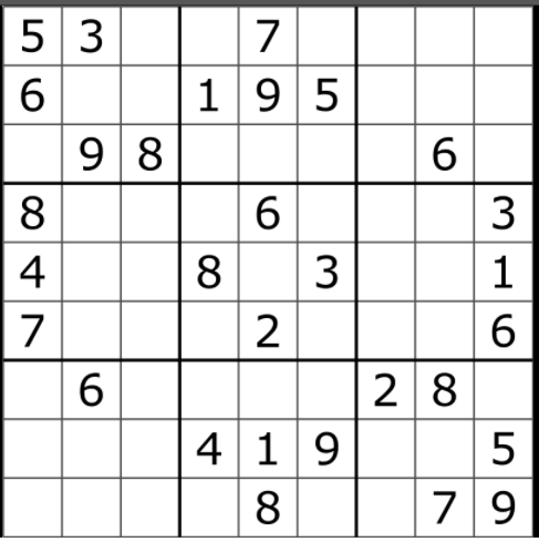
Format your output so that when your code prints out the result, it prints out the result in the shape of a sudoku puzzle:
-------------------------
| 5 3 . | . 7 . | . . . |
| 6 . . | 1 9 5 | . . . |
| . 9 8 | . . . | . 6 . |
-------------------------
| 8 . . | . 6 . | . . 3 |
| 4 . . | 8 . 3 | . . 1 |
| 7 . . | . 2 . | . . 6 |
-------------------------
| . 6 . | . . . | 2 8 . |
| . . . | 4 1 9 | . . 5 |
| . . . | . 8 . | . 7 9 |
-------------------------
Future Problem
use kNN to predict acceptance on sample college admissions dataset; compare with results from logistic regressor
Future Problem
Download sports prediction data (or movie prediction data), clean it up, make predictions using linear regression / logistic regression / Decision tree / random forest
Future Problem
boosting
Future Problem
KMeans class
Future Problem
5-neuron HH network on a graph
Future Problem
KMeans clustering by hand
Future Problem
DataFrame - left joins
Future Problem
Location: simulation/analysis/hebbian_learning.py
Grading: 10 points
Spike-timing dependent plasticity -- causal updates
$$\begin{align*} \dfrac{\textrm d w_{\textrm{pre},\textrm{post}}}{\textrm dt} &= \int_{\delta}^{-\delta} V_\textrm{post}(t) V_\textrm{pre}(t - \tau) \cdot \tau e^{-|\tau / 10 \, \textrm{ms}|} \, \textrm d\tau \end{align*}$$Future Problem
Location: simulation/analysis/hebbian_learning.py
Grading: 10 points
Update weight from presynaptic neuron to postsynaptic neuron.
Hebbian weight updates: fire together, wire together
$$ \dfrac{\textrm d w_{\textrm{pre},\textrm{post}}}{\textrm dt} = \int_{\delta}^{-\delta} V_\textrm{post}(t) V_\textrm{pre}(t - \tau) \cdot e^{-|\tau/10\, \textrm{ms}|} \, \textrm d\tau $$Future Problem
Location: simulation/analysis/different_network_types.py
Grading: 10 points
Generate raster plots for: small world, scale free, ...
Future Problem
PageRank by hand. Later, implement in directed graph.
https://www.coursera.org/lecture/networks-illustrated/pagerank-example-calculation-iSfuF
Future Problem
Location: simulation/analysis/10-neuron-network.py
Grading: 10 points
a. Simulate a 10-neuron network with connectivity $1 \to 2 \to 3 \to \cdots \to 10.$ You should get the following result:
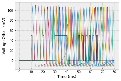
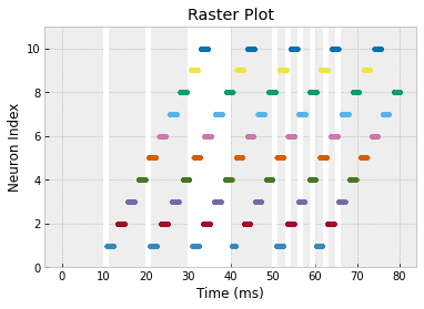
b. The plot above is really hard to interpret! So let's plot it a way that makes the most important information more clear. The most important information is when the neurons spiked. We'll say that a spike occurs whenever $V > 50 \, \textrm{mV}.$
To clearly display the spikes, let's change the $y$-axis to the neuron index and make a dot whenever $V > 50 \, \textrm{mV}.$ To show the electrode stimuli, let's color the plot white whenever the electrode is on.
To get the white background, you can plot a function that alternates between $0$ and $\textrm{max_neuron_index}+1$ whenever the electrode is on.
To plot dots, just pass
'.'as a parameter. To restrict the $y$-limits of the plot, useplt.ylim(min_y, max_y).
You should get the following result:
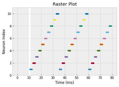
c. Find a network configuration that yields the following raster plot. Note that the stimulus has been changed so that it is just a single pulse at the beginning.
Future Problem
KFoldCrossValidator class - should work with kNearestNeighbors
Future Problem
PageRank
Future Problem
Constructing small-world & scale-free networks
Future Problem
neural net
Future Problem
NOTE: NEED TO MODIFY EULERESTIMATOR TO MAKE THIS EASIER TO IMPLEMENT
- what variables do we need to store, and what values of them do we need to store?
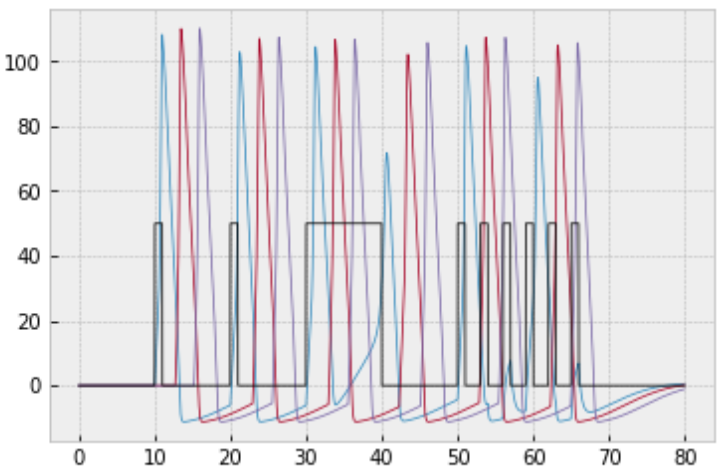
When a neuron fires, the action potential does not reach the synapse instantaneously. There is a small delay depending on how far away the synapse is. Let's say the delay is about $2 \, \textrm{ms}.$ Then we have
$$\dfrac{\textrm dV}{\textrm dt} = \underbrace{\dfrac{1}{C} \left[ s(t) - I_{\text{Na}}(t) - I_{\text K}(t) - I_{\text L}(t) \right]}_\text{neuron in isolation} + \underbrace{\dfrac{1}{C} \left( \sum\limits_{\begin{matrix} \textrm{synapses from} \\ \textrm{other neurons} \\ \textrm{with } V(t-2) > 50 \end{matrix}} V_{\text{other neuron}}(t-2) \right)}_\text{interactions with other neurons}.$$Taking the above changes into account, simulate 3 neurons connected in the fashion $1 \to 2 \to 3,$ where neuron $1$ receives the following electrode stimulus: $$ s(t) = \begin{cases} 50, & t \in [10,11] \cup [20,21] \cup [30,40] \cup [50,51] \cup [53,54] \\ & \phantom{t \in [} \cup [56,57] \cup [59,60] \cup [62,63] \cup [65,66] \\ 0 & \text{otherwise} \end{cases} $$
You should get the following result:
Future Problem
AND translate your pseudocode for your strategy into an actual strategy class for your strategy
Future Problem
SA, RHC, GA on 8 queens, TSP, knapsack
Future Problem
Simulated annealing & RHC on knapsack problem
Future Problem
Simulated annealing & RHC on TSP
Future Problem
simulated annealing; compare with RHC on 8 queens
Future Problem
A* search
Future Problem
solving sudoku puzzle using backtracking (the extra credit problem from first semester)
Future Problem
min-cut algorithm in weighted graph
Future Problem
Kruskal's algorithm in weighted graph
Future Problem
Weighted graph class using Dijkstra's algorithm for shortest path method
Future Problem
Euler estimator -- keep track of lag variables
generalize the idea of points -- a point takes the form point[variable_name][num_lookback_steps], where each component has a max number of lookback steps (defined upon intialization). Then we can reference in our derivatives: x['voltage1'][2/step_size] for delay; x['voltage2'][0] for no delay
Here, you will implement this and make sure it works with your SIR model. The new SIR model will assume it takes 1 week before it's possible to recover from the disease.
def dS_dt(t, x, step_size):
    susceptible = x['susceptible'][0]
    infected = x['infected'][0]
    return -0.0003 * susceptible * infected

def dI_dt(t, x, step_size):
    lookback_steps = round((1/52)/step_size)
    susceptible = x['susceptible'][0]
    infected = x['infected'][0]

    if len(x['infected']) > lookback_steps:
        infected_lookback = x['infected'][lookback_steps]
    else:
        infected_lookback = 0

    return 0.0003 * susceptible * infected - 0.02 * infected_lookback

def dR_dt(t, x, step_size):
    lookback_steps = round((1/52)/step_size)

    if len(x['infected']) > lookback_steps:
        infected_lookback = x['infected'][lookback_steps]
    else:
        infected_lookback = 0

    return 0.02 * infected_lookback

derivatives = {
    'susceptible': dS_dt,
    'infected': dI_dt,
    'recovered': dR_dt
}

max_lookback_times = {
    'susceptible': 0,
    'infected': 1/52,
    'recovered': 0
}

starting_point = (0, {'susceptible': [1000], 'infected': [1], 'recovered': [0]}) # NOTE THAT THE VALUES ARE NOW ARRAYS

estimator = EulerEstimator(derivatives, starting_point, max_lookback_times)
make a plot with 1 week minimum recovery period vs possible immediate recovery.
Future Problem
random forest
Future Problem
Random split decision tree
Future Problem
Normal distribution - estimate probabilities using left/right Riemann sums, midpoint rule, trapezoidal rule, Simpson's method
Future Problem
tables.query("""
    SELECT columnName1, columnName2, ..., columnNameN
    FROM tableName
    WHERE
        condition1 AND
        condition2 OR
        condition3 AND
        ...
        conditionM
    ORDER BY
        columnNameA ASC
        columnNameB DES
        columnNameC ASC
        ...
    """)
Future Problem
write SQL-like query language from scratch on dictionary of dataframes
first task:
tables.query("""
    SELECT columnName1, columnName2, ..., columnNameN
    FROM tableName
    ORDER BY
        columnNameA ASC
        columnNameB DES
        columnNameC ASC
        ...
    """)
Test (use Kaggle toy dataset)
df = DataFrame(
    ...
)
sql = SQLWorkspace({
    'words': words_df
})

sql.query
Future Problem
DataFrame.from_csv(filename)
Future Problem
Supplementary problems -- have C&M catch up on sqlzoo and probability for next assignment, so that both classes can share supplementary problems.
Make progress on these each time we don't have quiz corrections. Take screenshot of success, and paste your code into overleaf. Do 3 problems of each category. Synchronize it between classes (c&m can catch up in a day while ML does game refactoring)
- https://www.hackerrank.com/domains/cpp
- https://www.hackerrank.com/domains/shell
- https://sqlzoo.net/ (left off module 3 question 11)
I'll come up with some haskell problems to go along with the reading; start out here:
- http://learnyouahaskell.com/starting-out; put on repl.it (https://repl.it/new/haskell)
Include pics of problems - 2 each time (each from different chapter)
- Probability / statistics
- Operations research
Future Problem
asdf
Future Problem
Estimated Time: 20 minutes
Grade Weighting: 20%
Complete your code review. Submit links to the issues that you made. See the new code review procedure here: https://www.eurisko.us/resources/#code-reviews
Resolve 1 issue that has been made on your own code.
Future Problem
Exchange dumbplayer/combatplayer with classmates and make sure tests still pass. If any test doesn't pass, figure out whether it's your game's fault or the classmate's strategy's fault. If it's your game's fault, fix it.
Future Problem
Future Problem
Regular problem in which we take a dataset and do a prediction task using all the models we've built
Future Problem
single-layer perceptron
Future Problem
Random forest improvements
do it with a messier / more high-dimensional dataset
each tree only selects a subset of features
Future Problem
Write another test for decision tree with MANY features, much depth (?)
Future Problem
machine-learning/analysis/8_queens_hill_climbing.py
Solve the 8-queens problem using hill climbing, randomized hill climbing, and simulated annealing
Objective function: number of pairs of queens that are on same row, column, or diagonal
initialize randomly; move 1 queen 1 space
Randomized hill climbing: Repeatedly select a neighbor at random, and decides (based on the amount of improvement in that neighbor) whether to move to that neighbor or to examine another. For our purposes, use threshold = increase objective function by 2.
Random-restart hill climbing (aka "shotgun" hill climbing) - It iteratively does hill-climbing, each time with a random initial condition $x_{0}.$ The best $x_{m}$ is kept: if a new run of hill climbing produces a better $x_{m}$ than the stored state, it replaces the stored state.
run each 100 times; compute average running time; compute average ending value of the objective function; compare. Write up result in overleaf.
Plot each trial on same graph; really thin lines so all 300 can be overlaid
Future Problem
Finally, we'll refactor our random forest into a proper random forest
now that the trees are faster, we can afford to bring back gini. But we don't want to force
- random decision tree should select random feature, but we should still use the gini metric to find the best split in the randomly selected set of columns
put kNN and naive bayes and linear regressor in the comparison as well
Future Problem
random-restart hill climbing
simulated annealing
hash table
A* search
Dijkstra's algorithm
Future Problem
b. Create [YourNameHere]Player in [your_name_here]_player.py. In tests/test_[your_name_here]_player.py, ensure that your custom player beats both DumbPlayer and CombatPlayer.
On Wednesday's assignment, we'll conduct a practice tournament for everyone's players to compete.
- If you want to prepare your player for the tournament, you can conduct practice battles against your classmates over the weekend.
On Friday's assignment, we'll have the real first tournament
- The winner of the tournament will get an extra 20% on the assignment, and 2nd place will get an extra 10%.
Over the weekend, write up about how your strategy works and what kinds of problems you want to solve
Future Problem
Echo server
Run your analysis from 77-1 again, using max_depth=3 for all your decision trees. Post your results on #results, and state how long it took you to train the models now that you're using the max_depth setting.
b. test cases for random forest
Future Problem
socket connections -- build calculator
Future Problem
Create your custom strategy. Here is an example strategy that (I think) is really simple and doesn't do anything too dumb. Make sure that your custom strategy defeats it.
class ExampleStrategy:
    # buys as many scouts as possible and sends them directly
    # towards the opponent homeworld

    def __init__(self, player_index):
        self.player_index = player_index

    def will_colonize_planet(self, coordinates, hidden_game_state):
        return True

    def decide_ship_movement(self, unit_index, hidden_game_state):
        myself = hidden_game_state['players'][self.player_index]
        opponent_index = 1 - self.player_index
        opponent = hidden_game_state['players'][opponent_index]

        unit = myself['units'][unit_index]
        x_unit, y_unit = unit['coords']
        x_opp, y_opp = opponent['home_coords']

        translations = [(0,0), (1,0), (-1,0), (0,1), (0,-1)]
        best_translation = (0,0)
        smallest_distance_to_opponent = 999999999999
        for translation in translations:
            delta_x, delta_y = translation
            x = x_unit + delta_x
            y = x_unit + delta_y
            dist = abs(x - x_opp) + abs(y - y_opp)
            if dist < smallest_distance_to_opponent:
                best_translation = translation
                smallest_distance_to_opponent = dist

        return best_translation

    def decide_purchases(self, hidden_game_state):
        myself = hidden_game_state['players'][self.player_index]
        cp = myself['cp']

        homeworld_coords = [unit['coords'] for unit in myself['units'] if unit['type'] == 'Homeworld'][0]
        shipsize_tech_level = myself['technology']['shipsize']
        hullsize_capacity_per_shipyard = 0.5 + 0.5 * shipsize_tech_level
        shipyards_at_homeworld = [unit for unit in myself['units'] if unit['type'] == 'Shipyard' and unit['coords'] == homeworld_coords]
        hullsize_capacity = hullsize_capacity_per_shipyard * len(shipyards_at_homeworld)

        scout_data = hidden_game_state['unit_data']['Scout']
        scout_cost = scout_data['cp_cost']
        scout_hullsize = scout_data['hullsize']

        purchases = {'units': [], 'technology': []}
        while cp > scout_cost and hullsize_capacity > scout_hullsize:
            pair = ('Scout', homeworld_coords)
            purchases['units'].append(pair)

        return purchases

    def decide_removal(self, hidden_game_state):
        # remove unit that's furthest from enemy

        myself = hidden_game_state['players'][self.player_index]
        opponent_index = 1 - player_index
        opponent = hidden_game_state['players'][opponent_index]
        x_opp, y_opp = opponent['home_coords']

        furthest_unit_index = 0
        furthest_distance_to_opponent = 999999999999
        for unit_index, unit in enumerate(myself['units']):
            x_unit, y_unit = unit['coords']
            dist = abs(x_unit - x_opp) + abs(y_unit - y_opp)
            if dist > furthest_distance_to_opponent:
                furthest_unit_index = unit_index
                furthest_distance_to_opponent = dist

        return furthest_unit_index

    def decide_which_unit_to_attack(self, hidden_game_state_for_combat, combat_state, coords, attacker_index):
        # attack opponent's first ship in combat order

        combat_order = combat_state[coords]
        player_indices = [unit['player_index'] for unit in combat_order]

        opponent_index = 1 - self.player_index
        for combat_index, unit in enumerate(combat_order):
            if unit['player_index'] == opponent_index:
                return combat_index

    def decide_which_units_to_screen(self, hidden_game_state_for_combat, combat_state, coords):

        combat_order = combat_state[coords]
        opponent_index = 1 - self.player_index
        player_indices = [unit['player_index'] for unit in combat_order]

        num_own_ships = len([n for n in player_indices if n == self.player_index])
        num_opponent_ships = len([n for n in player_indices if n == opponent_index])
        max_num_to_screen = max(0, num_own_ships - num_opponent_ships)

        indices_of_own_ships = [i for i,unit in enumerate(combat_order) if unit['player_index'] == self.player_index]

        return indices_of_own_ships[-max_num_to_screen:]
Future Problem
https://www.learncpp.com/ -- start with ch9
Future Problem
Fix this problem to use vectors
Implementation instructions:
Even if you know a more mathematically elegant way to implement this function, please do it according to the following specifications. The goal is to give you some practice working with arrays.
Helper functions:
Create a recursive function
kthFibonacciNumber(int k)that computes thekth Fibonacci number.Create a function
kthPartialSum(int k)that creates an
computes the sum of the first k Fibonacci numbers.
Then, in the primary function metaFibonacciSum(int n):
Create an array containing the Fibonacci numbers $a_0, a_1, ..., a_n.$
Create an array containing the partial sums $S_{a_0}, S_{a_1}, ..., S_{a_n}.$
Compute the sum of the partial sums array.
Helpful resource: https://www.learncpp.com/cpp-tutorial/arrays-and-loops/
Code template:
# include <iostream>
# include <cassert>

int kthFibonacciNumber(int k)
{
    // your code here
}

int kthPartialSum(int k)
{
    // your code here
}

int metaFibonacciSum(int n)
{
    // your code here
}

int main()
{
    std::cout << "Testing...\n";

    assert(metaFibonacciSum(6) == 74);

    std::cout << "Success!";

    return 0;
}
Debugging note: A failed assert will obliterate any messages that would otherwise be printed out on the same line. So if you want a message to print even in the event of a failed assert, you have to put \n at the end of it so that the assert gets moved to the next line of output.
#include <iostream>
#include <cassert>
int main()
{
    std::cout << "This line will print\n";
    assert(2+2==5);
}
#include <iostream>
#include <cassert>
int main()
{
std::cout << "This line will NOT print";
assert(2+2==5);
}Future Problem
strategy problem writeup; prepare for meeting with Prof. Wierman
8 queens -- random restart hill climbing
game level 3 implementation
randomized hill climbing applied to game level 3 (too many possibilities to simulate them all)
Future Problem
neural net with hidden layer and rectified linear units (ReLUs)
Future Problem
generalize neural net to any number of inputs & any number of outputs
then fit the sandwich dataset with linear and logistic neural nets
extend hash table
Game level 4
- Colonization, with 2 planets in middle of board but on opposite sides
Future:
- other ship types, miners, scuttling, screening
Future Problem
Intro to linear programming
Problem 97-1
This problem is the beginning of some more involved machine learning tasks. To ease the transition, this will be the only problem on this assignment.
This problem is just as important as space empires and neural nets, and the modeling techniques covered will 100% be on future quizzes and the final. Be sure to do this problem well. If you've run into any issues with your space empires simulations, DO THIS PROBLEM FIRST before you go back to space empires.
Make an account on Kaggle.com so that we can walk through a Titanic prediction task.
Go to https://www.kaggle.com/c/titanic/data, scroll down to the bottom, and click "download all". You'll get a zip file called
titanic.zip.Upload
titanic.zipintomachine-learning/datasets/titanic/. Then, rununzip machine-learning/datasets/titanic/titanic.zipin the command line to unzip the file.This gives us 3 files:
train.csv,test.csv, andgender_submission.csv. The filetrain.csvcontains data about a bunch of passengers along with whether or not they survived. Our goal is to usetrain.csvto build a model that will predict the outcome of passengers intest.csv(for which the survival data is not given).IMPORTANT: To prevent confusion, rename
train.csvtodataset_of_knowns.csv, renametest.csvtounknowns_to_predict.csv, and renamegender_submission.csvtopredictions_from_gender_model.csv.The file
predictions_from_gender_model.csvis an example of predictions from a really, really basic model: if the passenger is female, predict that they survived; if the passenger is male, predicte that they did not survive.
To build a model, we will proceed with the following steps:
Feature Selection - deciding which variables we want in our model. This is usually a subset of the original number of features.
Model Selection - ranking our models from best to worst, based on cross-validation performance. (We'll train each model on half the data, use it to predict the other half of the data, and see how accurate it is.)
Submission - taking our best model, training it on the full
dataset_of_knowns.csv, running it onunknowns_to_predict.csv, generating apredictions.csvfile, and uploading it to Kaggle.com for scoring.
For this problem, you will need to write what you did for each of these steps in an Overleaf doc (kind of like you would in a lab journal). So, open up one now and let's continue.
Feature Engineering
In your Overleaf doc, create a section called "Feature Selection". Make a bulleted list of all the features along with your justification for using or not using the feature in your model.
Important: There is a data dictionary at https://www.kaggle.com/c/titanic/data that describes what each feature means.
It will be helpful to look at the actual values of the variables as well. For example, here are the first 5 records in the dataset:
PassengerId,Survived,Pclass,Name,Sex,Age,SibSp,Parch,Ticket,Fare,Cabin,Embarked
1,0,3,"Braund, Mr. Owen Harris",male,22,1,0,A/5 21171,7.25,,S
2,1,1,"Cumings, Mrs. John Bradley (Florence Briggs Thayer)",female,38,1,0,PC 17599,71.2833,C85,C
3,1,3,"Heikkinen, Miss. Laina",female,26,0,0,STON/O2. 3101282,7.925,,S
4,1,1,"Futrelle, Mrs. Jacques Heath (Lily May Peel)",female,35,1,0,113803,53.1,C123,S
5,0,3,"Allen, Mr. William Henry",male,35,0,0,373450,8.05,,S
For every feature that you decide to keep, give a possible theory for how the feature may help predict whether a passenger survived.
- For example, you should keep the
Agefeature because it's likely that younger passengers were given priority when boarding lifeboats.
For every feature that you decide to remove, explain why it 1) is irrelevant to the prediction task, or 2) would take too long to transform into a worthwhile feature.
- For example, you can remove the
ticketfeature because it's formatted so weirdly (e.g.A/5 21171). It's possible that there may be some information here, but it would take a while to figure out how to turn this into a worthwhile feature that we could actually plug into our model. (There's multiple parts to the ticket number and it's a combination of letters and numbers, so it's not straightforward how to use it.)
Model Selection
Split dataset_of_knowns.csv in half, selecting every other row for training and leaving the leftover rows for testing.
Fit several models to the training dataset:
Linear regressor - if output is greater than or equal to 0.5, predict category 1 (survived); if output is less than 0.5, predict category 0 (didn't survive). You may wish to include interaction terms that you think would be important, since linear regressors do not capture interactions by default.
Logistic regressor - same notes as above (for the linear regressor)
Gini decision tree - conveniently, decision trees predict categorical variables by default ("survived" has 2 categories, 0 and 1), and they also capture interactions by default (so don't include any interaction terms when you feed the data into the Gini tree). We'll try out 2 different models, one with
max_depth=5and another withmax_depth=10.Random forest - same notes as above (for the Gini decision tree). We'll try out 2 different models, one with
max_depth=3andnum_trees=1000, and another withmax_depth=5andnum_trees=1000.Naive Bayes - note that you'll need to take any features that are quantitative and re-label their values by categories. By default, you can just use 3 categories: "low", "mid", "high", where the lowest third of the data is re-labeled with the category "low", the highest third of the data is re-labeled with the category "high", and the middle third of the data is re-labeled with the category "mid".
- For example, suppose you had a variable that had values
[1,4,3,3,2,5,7,6,4]. Sorted, these values are[1,2,3,3,4,4,5,6,7]. So we'd relabel1,2,3as"low",5,6,7as"high", and4as"mid". So, the values[1,4,3,3,2,5,7,6,4]would get transformed into["low","mid","low","low","low","high","high","high","mid"]
- For example, suppose you had a variable that had values
k-Nearest Neighbors - for any variables that are quantitative, transform them as $$ x \to \dfrac{x - \min(x)}{\max(x) - \min(x)} $$ so that they fit into the interval
[0,1].For any variables that are categorical, leave them be. Use a "Mahnattan" distance metric (the sum of absolute differences). Note that if a variable is categorical, then their distance between 2 values should be counted as $0$ if they are the same and $1$ if they are different. We'll try 2 different models,k=5andk=10.The reason for the Manhattan distance metric instead of the Euclidean distance metric is so that differences between categorical variables do not drastically overpower differences between quantitative variables.
For example, suppose you had two data points
(0.2, 0.7, "dog", "red")and(0.5, 0.1, "cat", "red"). Then the distance would be as follows:distance = |0.2-0.5| + |0.7-0.1| + int("dog"!="cat") + int("red"!="red") = 0.3 + 0.6 + 1 + 0 = 1.9
Then, use these models to predict survival for the training dataset and the testing dataset separately. Make a table in your Overleaf doc that contains the resulting accuracy rates.
- For example, suppose there are 100 rows in the training dataset and 100 rows in the testing dataset (to be clear, the actual number of rows in your dataset will probably be different). You train your Gini decision tree with
max_depth=10on the training dataset, and then use it to predict on the testing dataset. You get 98 correct predictions on the training dataset and 70 correct predictions on the testing dataset (which, by the way, is an indication that you're overfitting -- yourmax_depthis probably too high). Then your table looks like this:
Model         | Training Accuracy | Testing Accuracy
----------------------------------------------------------
Gini depth 10 | 98%               | 70%
To be clear, your table should have 9 rows, one for each model: linear, logistic, Gini depth 5, Gini depth 10, random forest depth 5, random forest depth 10, naive Bayes, 5-nearest-neighbors, 10-nearest-neighbors.
Submission
Take your best model (i.e. the one with the highest testing accuracy) and evaluate its predictions on unknowns_to_predict.csv.
Save your results as predictions.csv, and make sure they follow the exact same format as predictions_from_gender_model.csv.
- By "the exact same format", I mean THE EXACT SAME FORMAT. Make sure the header is exactly the same. Make sure that you're writing the
0's and1s as integers, not strings. Make sure that you include thePassengerIdcolumn. Make sure that the values in thePassengerIdcolumn match up exactly with those inpredictions_from_gender_model.csv. The only thing that should be different is the values in theSurvivedcolumn.
Click on the "Submit Predictions" button on the right side of the screen and submit your file predictions.csv. You should get a screen that looks like the image below, but has your predictions.csv instead of gender-submissions.csv. You should also get a higher score than 0.76555 (which is the baseline accuracy of the gender model).

Take a screenshot of this screen, post it on #machine-learning, and include it in your Overleaf writeup.
What to Turn In
Just the Overleaf writeup and a commit link to your machine-learning repo. That's it.
Problem 96-1
Space Empires
Once your strategy is finalized, Slack it to me and I'll upload it here.
https://github.com/eurisko-us/eurisko-us.github.io/tree/master/files/strategies/cohort-1/level-3
Then, once everyone's strategies are submitted, I'll make an announcement, and you can download the strategies from the above folder and run all pairwise battles for 100 games.
Go through
max_turns=100before declaring a draw. I think this should run quick enough, since we decreased from 500 games to 100 games, but if any 100-game matchups are taking longer than a couple minutes to run, then post about it and we'll figure something out.Put your data in the spreadsheet:
https://docs.google.com/spreadsheets/d/1zUqn5OvF3_U3XJ_d25vtBiFkRB3RgSQSXNv6wga8aeI/edit?usp=sharing
Remember to switch the order of the players halfway through the simulation so that each player goes first an equal number of times.
Seed the games: game 1 has seed 1, game 2 has seed 2, and so on. This way, we should all get exactly the same results.
As usual, there will be prizes:
- 1st place: 50 pts extra credit in the assignments category
- 2nd place: 30 pts extra credit in the assignments category
- 3rd place: 10 pts extra credit in the assignments category
Neural Nets
Compute $\dfrac{\textrm dE}{\textrm dw_{34}},$ $\dfrac{\textrm dE}{\textrm dw_{24}},$ $\dfrac{\textrm dE}{\textrm dw_{13}},$ $\dfrac{\textrm dE}{\textrm dw_{12}},$ and $\dfrac{\textrm dE}{\textrm dw_{01}}$ for the following network. (It's easiest to do it in that order.) Put your work in an Overleaf doc.
$$ \begin{matrix} & & n_4 \\ & \nearrow & & \nwarrow \\ n_2 & & & & n_3 \\ & \nwarrow & & \nearrow \\ & & n_1 \\ & & \uparrow \\ & & n_0 \\ \end{matrix} $$Show ALL your work! Also, make sure to use the simplest notation possible (for example, instead of writing $f_k(i_k),$ write $a_k$)
Check your answer by substituting the following values:
$$ y_\textrm{actual}=1 \qquad \begin{matrix} a_0 = 2 \\ a_1 = 3 \\ a_2 = 4 \\ a_3 = 5 \\ a_4 = 6 \end{matrix} \qquad \begin{matrix} f_0'(i_0) = 7 \\ f_1'(i_1) = 8 \\ f_2'(i_2) = 9 \\ f_3'(i_3) = 10 \\ f_4'(i_4) = 11 \end{matrix} \qquad \begin{matrix} w_{01} = 12 \\ w_{12} = 13 \\ w_{13} = 14 \\ w_{24} = 15 \\ w_{34} = 16 \end{matrix} $$You should get $$ \dfrac{\textrm dE}{\textrm d w_{34}} = 550, \qquad \dfrac{\textrm dE}{\textrm d w_{24}} = 440, \qquad \dfrac{\textrm dE}{\textrm d w_{13}} = 52800, \qquad \dfrac{\textrm dE}{\textrm d w_{12}} = 44550, \qquad \dfrac{\textrm dE}{\textrm d w_{01}} = 7031200. $$
Problem 96-2
Haskell
Write a recursive function merge that merges two sorted lists. To do this, you can check the first elements of each list, and make the lesser one the next element, then merge the lists that remain.
merge (x:xs) (y:ys) = if x < y
                        then _______
                        else _______
merge [] xs = ____
merge xs [] = ____

main = print(merge [1,2,5,8] [3,4,6,7,10])
-- should return [1,2,3,4,5,6,7,8,10]
SQL
On sqltest.net, create a sql table by copying the following script:
Then, compute the average assignment score of each student. List the results from highest to lowest, along with the full names of the students.
This is what your output should look like:
fullname    avgScore
Ishmael Smith   90.0000
Sylvia Sanchez  86.6667
Kinga Shenko    85.0000
Franklin Walton 80.0000
Harry Ng    78.3333
Hint: You'll have to use a join and a group by.
Problem 96-3
Commit + Review
Commit your code to Github.
Make 1 GitHub issue on your assigned classmate's repository (but NOT
assignment-problems). See eurisko.us/resources/#code-reviews to determine your assigned classmate.
(You don't have to resolve any issues on this assignment)
Submission Template
For your submission, copy and paste your links into the following template:
neural nets overleaf: _____
put your game results in the spreadsheet (but you don't have to paste the link)
Repl.it link to haskell file: _____
sqltest.net link: _____

commits: _____
(space-empires, assignment-problems)

Created issue: _____
Problem 95-1
Neural Nets
Notation
$n_k$ - the $k$th neuron
$a_k$ - the activity of the $k$th neuron
$i_k$ - the input to the $k$th neuron. This is the weighted sum of activities of the parents of $n_k.$ If $n_k$ has no parents, then $i_k$ comes from the data directly.
$f_k$ - the activation function of the $k$th neuron. Note that in general, we have $a_k = f_k(i_k)$
$w_{k \ell}$ - the weight of the connection $n_k \to n_\ell.$ In your code, this is
weights[(k,l)].$E = (y_\textrm{predicted} - y_\textrm{actual})^2$ is the squared error that results from using the neural net to predict the value of the dependent variable, given values of the independent variables
$w_{k \ell} \to w_{k \ell} - \alpha \dfrac{\textrm dE}{\textrm dw_{k\ell}}$ is the gradient descent update, where $\alpha$ is the learning rate
Example
For a simple network $$ \begin{matrix} & & n_2 \\ & \nearrow & & \nwarrow \\ n_0 & & & & n_1,\end{matrix} $$ we have:
$$\begin{align*} y_\textrm{predicted} &= a_2 \\ &= f_2(i_2) \\ &= f_2(w_{02} a_0 + w_{12} a_1) \\ &= f_2(w_{02} f_0(i_0) + w_{12} f_1(i_1) ) \\ \\ \dfrac{\textrm dE}{\textrm dw_{02}} &= \dfrac{\textrm d}{\textrm dw_{02}} \left[ (y_\textrm{predicted} - y_\textrm{actual})^2 \right] \\ &= \dfrac{\textrm d}{\textrm dw_{02}} \left[ (a_2 - y_\textrm{actual})^2 \right] \\ &= 2(a_2 - y_\textrm{actual}) \dfrac{\textrm d}{\textrm dw_{02}} \left[ a_2 - y_\textrm{actual} \right] \\ &= 2(a_2 - y_\textrm{actual}) \dfrac{\textrm d }{\textrm dw_{02}} \left[ a_2 \right] \\ &= 2(a_2 - y_\textrm{actual}) \dfrac{\textrm d }{\textrm dw_{02}} \left[ f_2(i_2) \right] \\ &= 2(a_2 - y_\textrm{actual}) f_2'(i_2) \dfrac{\textrm d }{\textrm dw_{02}} \left[ i_2 \right] \\ &= 2(a_2 - y_\textrm{actual}) f_2'(i_2) \dfrac{\textrm d }{\textrm dw_{02}} \left[ w_{02} a_0 + w_{12} a_1 \right] \\ &= 2(a_2 - y_\textrm{actual}) f_2'(i_2) \dfrac{\textrm d }{\textrm dw_{02}} \left[ w_{02} a_0 + w_{12} a_1 \right] \\ &= 2(a_2 - y_\textrm{actual}) f_2'(i_2) a_0 \\ \\ \dfrac{\textrm dE}{\textrm dw_{12}} &= 2(a_2 - y_\textrm{actual}) f_2'(i_2) a_1 \end{align*}$$THE ACTUAL PROBLEM STATEMENT
Compute $\dfrac{\textrm dE}{\textrm dw_{23}},$ $\dfrac{\textrm dE}{\textrm dw_{12}},$ and $\dfrac{\textrm dE}{\textrm dw_{01}}$ for the following network. (It's easiest to do it in that order.) Put your work in an Overleaf doc.
$$ \begin{matrix} n_3 \\ \uparrow \\ n_2 \\ \uparrow \\ n_1 \\ \uparrow \\ n_0 \end{matrix} $$Show ALL your work! Also, make sure to use the simplest notation possible (for example, instead of writing $f_k(i_k),$ write $a_k$)
Check your answer by substituting the following values:
$$ y_\textrm{actual}=1 \qquad \begin{matrix} a_0 = 2 \\ a_1 = 3 \\ a_2 = 4 \\ a_3 = 5 \end{matrix} \qquad \begin{matrix} f_0'(i_0) = 6 \\ f_1'(i_1) = 7 \\ f_2'(i_2) = 8 \\ f_3'(i_3) = 9 \end{matrix} \qquad \begin{matrix} w_{01} = 10 \\ w_{12} = 11 \\ w_{23} = 12 \end{matrix} $$You should get $$ \dfrac{\textrm dE}{\textrm d w_{23}} = 288, \qquad \dfrac{\textrm dE}{\textrm d w_{12}} = 20736, \qquad \dfrac{\textrm dE}{\textrm d w_{01}} = 1064448. $$
Note: On the next couple assignments, we'll do the same exercise with progressively more advanced networks. This problem is relatively simple so that you have a chance to get used to working with the notation.
Space Empires
Finish creating your game level 3 strategy. (See problem 93-1 for a description of game level 3, which you should have implemented by now.) Then, implement the following strategy and run it against your level 3 strategy:
NumbersBerserkerLevel3- always buys as many scouts as possible, and each time it buys a scout, immediately sends it on a direct route to attack the opponent.
Post on #machine-learning with your strategy's stats against these strategies:
MyStrategy vs NumbersBerserker
- MyStrategy win rate: __%
- MyStrategy loss rate: __%
- draw rate: __%
On the next assignment, we'll have the official matchups.
Problem 95-2
C++
Write a function calcSum(m,n) that computes the sum of the matrix product of an ascending $m \times n$ and a descending $n \times m$ array, where the array entries are taken from $\{ 1, 2, ..., mn \}.$ For example, if $m=2$ and $n=3,$ then
#include <iostream>
#include <cassert>

// define calcSum

int main() {
    // write an assert for the test case m=2, n=3
}
SQL
On sqltest.net, create the following tables:
CREATE TABLE age (
id INT(6) UNSIGNED AUTO_INCREMENT PRIMARY KEY,
lastname VARCHAR(30),
age VARCHAR(30)
);

INSERT INTO `age` (`id`, `lastname`, `age`)
VALUES ('1', 'Walton', '12');

INSERT INTO `age` (`id`, `lastname`, `age`)
VALUES ('2', 'Sanchez', '13');

INSERT INTO `age` (`id`, `lastname`, `age`)
VALUES ('3', 'Ng', '14');

INSERT INTO `age` (`id`, `lastname`, `age`)
VALUES ('4', 'Smith', '15');

INSERT INTO `age` (`id`, `lastname`, `age`)
VALUES ('5', 'Shenko', '16');

CREATE TABLE name (
id INT(6) UNSIGNED AUTO_INCREMENT PRIMARY KEY,
firstname VARCHAR(30),
lastname VARCHAR(30)
);

INSERT INTO `name` (`id`, `age`, `lastname`)
VALUES ('1', 'Franklin', 'Walton');

INSERT INTO `name` (`id`, `firstname`, `lastname`)
VALUES ('2', 'Sylvia', 'Sanchez');

INSERT INTO `name` (`id`, `firstname`, `lastname`)
VALUES ('3', 'Harry', 'Ng');

INSERT INTO `name` (`id`, `firstname`, `lastname`)
VALUES ('4', 'Ishmael', 'Smith');

INSERT INTO `name` (`id`, `firstname`, `lastname`)
VALUES ('5', 'Kinga', 'Shenko');
Then, write a query to get the full names of the people, along with their ages, in alphabetical order of last name. The output should look like this:
Harry Ng is 14.
Sylvia Sanchez is 13.
Kinga Shenko is 16.
Ishmael Smith is 15.
Franklin Walton is 12.
Tip: You'll need to use string concatenation and a join.
Problem 95-3
Commit + Review
Commit your code to Github.
Make 1 GitHub issue on your assigned classmate's repository (but NOT
assignment-problems). See eurisko.us/resources/#code-reviews to determine your assigned classmate.
(You don't have to resolve any issues on this assignment)
Submission Template
For your submission, copy and paste your links into the following template:
Overleaf: _____
Repl.it link to C++ file: _____
sqltest.net link: _____

assignment-problems commit: _____
space-empires commit: _____

Created issue: _____
Problem 94-1
Space Empires
Reconcile remaining discrepancies in game level 2 so we can crown the winners:
https://docs.google.com/spreadsheets/d/1zUqn5OvF3_U3XJ_d25vtBiFkRB3RgSQSXNv6wga8aeI/edit?usp=sharing
Then, write your first custom strategy for the level 3 game. We'll start matchups on Wednesday. We'll go through several rounds of matchups on this level since the game is starting to become more rich.
(We'll have the same extra credit prizes for 1st / 2nd / 3rd place)
Note: In decide_which_unit_to_attack, be sure to use 'player' and 'unit' instead of 'player_index' and 'unit_index'.
# combat_state is a dictionary in the form coordinates : combat_order
        # {
        #    (1,2): [{'player': 1, 'unit': 0},
        #            {'player': 0, 'unit': 1},
        #            {'player': 1, 'unit': 1},
        #            {'player': 1, 'unit': 2}],
        #    (2,2): [{'player': 2, 'unit': 0},
        #            {'player': 3, 'unit': 1},
        #            {'player': 2, 'unit': 1},
        #            {'player': 2, 'unit': 2}]
        # }
Neural Net-Based Logistic Regressor
Make sure you get this problem done completely. Neural nets have a very steep learning curve and they're going to be sticking with us until the end of the semester.
a. Given $\sigma(x) = \dfrac{1}{1+e^{-x}},$ prove that $\sigma'(x) = \sigma(x) (1-\sigma(x)).$ Write this proof in an Overleaf doc.
b. In neural networks, neurons are often given "activation functions", where
node.activity = node.activation_function(weighted sum of inputs to node)In this problem, you'll extend your neural net to include activation functions. Then, you'll equip the neurons with activations so as to implement a logistic regressor.
>>> weights = {(0,2): -0.1, (1,2): 0.5}

>>> def linear_function(x):
        return x
>>> def linear_derivative(x):
        return 1
>>> def sigmoidal_function(x):
        return 1/(1+math.exp(-x))
>>> def sigmoidal_derivative(x):
        s = sigmoidal_function(x)
        return s * (1 - s)

>>> activation_types = ['linear', 'linear', 'sigmoidal']
>>> activation_functions = {
    'linear': {
        'function': linear_function,
        'derivative': linear_derivative
    },
    'sigmoidal': {
        'function': sigmoidal_function,
        'derivative': sigmoidal_derivative
    }
}

>>> nn = NeuralNetwork(weights, activation_types, activation_functions)

>>> data_points = [
    {'input': [1,0], 'output': [0.1]},
    {'input': [1,1], 'output': [0.2]},
    {'input': [1,2], 'output': [0.4]},
    {'input': [1,3], 'output': [0.7]}
    ]
>>> for i in range(1,10001):
        err = 0
        for data_point in data_points:
            nn.update_weights(data_point)
            err += nn.calc_squared_error(data_point)
        if i < 5 or i % 1000 == 0:
            print('iteration {}'.format(i))
            print('    gradient: {}'.format(nn.calc_gradient(data_point))
            print('    updated weights: {}'.format(nn.weights))
            print('    error: {}'.format(err))
            print()

iteration 1
    gradient: {(0, 2): 0.03184692266577955, (1, 2): 0.09554076799733865}
    updated weights: {(0, 2): -0.10537885784041535, (1, 2): 0.4945789883636697}
    error: 0.40480006957774683

iteration 2
    gradient: {(0, 2): 0.031126202300065627, (1, 2): 0.09337860690019688}
    updated weights: {(0, 2): -0.11072951375555531, (1, 2): 0.48919868238711295}
    error: 0.3989945995186133

iteration 3
    gradient: {(0, 2): 0.030367826123201307, (1, 2): 0.09110347836960392}
    updated weights: {(0, 2): -0.11605116651884796, (1, 2): 0.4838609744178689}
    error: 0.3932640005281893

iteration 4
    gradient: {(0, 2): 0.029572207383720784, (1, 2): 0.08871662215116236}
    updated weights: {(0, 2): -0.12134303561025003, (1, 2): 0.4785677220228999}
    error: 0.3876106111541695

iteration 1000
    gradient: {(0, 2): -0.04248103992359947, (1, 2): -0.12744311977079842}
    updated weights: {(0, 2): -1.441870816044744, (1, 2): 0.6320712307086241}
    error: 0.03103391055967604

iteration 2000
    gradient: {(0, 2): -0.026576913835657988, (1, 2): -0.07973074150697396}
    updated weights: {(0, 2): -1.8462575194764488, (1, 2): 0.8112377281576201}
    error: 0.010469324799663702

iteration 3000
    gradient: {(0, 2): -0.019389915442213898, (1, 2): -0.058169746326641694}
    updated weights: {(0, 2): -2.0580006793189596, (1, 2): 0.903267622168482}
    error: 0.004993174823452696

iteration 4000
    gradient: {(0, 2): -0.01536481706566838, (1, 2): -0.04609445119700514}
    updated weights: {(0, 2): -2.187017035077964, (1, 2): 0.9588032475551099}
    error: 0.002982405174006053

iteration 5000
    gradient: {(0, 2): -0.012858896793162088, (1, 2): -0.038576690379486266}
    updated weights: {(0, 2): -2.2717393677429842, (1, 2): 0.995065996436664}
    error: 0.00211991513136444

iteration 6000
    gradient: {(0, 2): -0.011201146193726709, (1, 2): -0.033603438581180124}
    updated weights: {(0, 2): -2.3298248394321606, (1, 2): 1.0198377357361068}
    error: 0.0017156674543843792

iteration 7000
    gradient: {(0, 2): -0.010062009597155228, (1, 2): -0.030186028791465685}
    updated weights: {(0, 2): -2.370740520022862, (1, 2): 1.037244660012689}
    error: 0.0015153961429219282

iteration 8000
    gradient: {(0, 2): -0.009259319779522148, (1, 2): -0.027777959338566444}
    updated weights: {(0, 2): -2.400083365137227, (1, 2): 1.0497070597284772}
    error: 0.0014124679719747604

iteration 9000
    gradient: {(0, 2): -0.008683873946383038, (1, 2): -0.026051621839149115}
    updated weights: {(0, 2): -2.4213875864199608, (1, 2): 1.058744505427183}
    error: 0.0013582149901490035

iteration 10000
    gradient: {(0, 2): -0.00826631063707707, (1, 2): -0.024798931911231212}
    updated weights: {(0, 2): -2.4369901278483534, (1, 2): 1.065357551487286}
    error: 0.001329102258719855

>>> nn.weights
should be close to
    {(0,2): -2.44, (1,2): 1.07}

because the data points all lie approximately on the sigmoid
    output = 1/(1 + e^(-(input[0] * -2.44 + input[1] * 1.07)) )
Super Important: You'll have to update your gradient descent to account for the activation functions. This will require using the chain rule. In our case, we'll have
squared_error = (y_predicted - y_actual)^2

d(squared_error)/d(weights)
    = 2 (y_predicted - y_actual) d(y_predicted - y_actual)/d(weights)
    = 2 (y_predicted - y_actual) [ d(y_predicted)/d(weights) - 0]
    = 2 (y_predicted - y_actual) d(y_predicted)/d(weights)

y_predicted
    = nodes[2].activity
    = nodes[2].activation_function(nodes[2].input)
    = nodes[2].activation_function(
        weights[(0,2)] * nodes[0].activity
        + weights[(1,2)] * nodes[1].activity
    )
    = nodes[2].activation_function(
        weights[(0,2)] * nodes[0].activation_function(nodes[0].input)
        + weights[(1,2)] * nodes[1].activation_function(nodes[1].input)
    )

d(y_predicted)/d(weights[(0,2)])
    = nodes[2].activation_derivative(nodes[2].input)
       * d(nodes[2].input)/d(weights[(0,2)])
    = nodes[2].activation_derivative(nodes[2].input)
      * d(weights[(0,2)] * nodes[0].activity + weights[(1,2)] * nodes[1].activity)/d(weights[(0,2)])
    = nodes[2].activation_derivative(nodes[2].input)
       * nodes[0].activity

by the same reasoning as above:

d(y_predicted)/d(weights[(1,2)]
    = nodes[2].activation_derivative(nodes[2].input)
       * nodes[1].activity
Note: If no activation_functions variable is passed in, then assume all activation functions are linear.
Problem 94-2
HashTable
Write a class HashTable that generalizes the hash table you previously wrote. This class should store an array of buckets, and the hash function should add up the alphabet indices of the input string and mod the result by the number of buckets.
>>> ht = HashTable(num_buckets = 3)
>>> ht.buckets
[[], [], []]
>>> ht.hash_function('cabbage')
2    (because 2+0+1+1+0+6+4 mod 3 = 14 mod 3 = 2)

>>> ht.insert('cabbage', 5)
>>> ht.buckets
[[], [], [('cabbage',5)]]

>>> ht.insert('cab', 20)
>>> ht.buckets
[[('cab', 20)], [], [('cabbage',5)]]

>>> ht.insert('c', 17)
>>> ht.buckets
[[('cab', 20)], [], [('cabbage',5), ('c',17)]]

>>> ht.insert('ac', 21)
>>> ht.buckets
[[('cab', 20)], [], [('cabbage',5), ('c',17), ('ac', 21)]]

>>> ht.find('cabbage')
5
>>> ht.find('cab')
20
>>> ht.find('c')
17
>>> ht.find('ac')
21
SQL
This is a really quick problem, mostly just getting you to learn the ropes of the process we'll be using for doing SQL problems going forward (now that we're done with SQL Zoo).
On https://sqltest.net/, create table with the following script:
CREATE TABLE people (
id INT(6) UNSIGNED AUTO_INCREMENT PRIMARY KEY,
name VARCHAR(30) NOT NULL,
age VARCHAR(50)
);

INSERT INTO `people` (`id`, `name`, `age`)
VALUES ('1', 'Franklin', '12');

INSERT INTO `people` (`id`, `name`, `age`)
VALUES ('2', 'Sylvia', '13');

INSERT INTO `people` (`id`, `name`, `age`)
VALUES ('3', 'Harry', '14');

INSERT INTO `people` (`id`, `name`, `age`)
VALUES ('4', 'Ishmael', '15');

INSERT INTO `people` (`id`, `name`, `age`)
VALUES ('5', 'Kinga', '16');
Then select all teenage people whose names do not start with a vowel, and order by oldest first.
In order to run the query, you need to click the "Select Database" dropdown in the very top-right corner (so top-right that it might partially run off your screen) and select MySQL 5.6.
This is what your result should be:
id  name    age
5   Kinga   16
3   Harry   14
2   Sylvia  13
Copy the link where it says "Link for sharing your example:". This is what you'll submit for your assignment.
Problem 94-3
There will be a quiz on Friday over things that we've done with C++, Haskell, SQL, and Neural Nets.
Commit + Review
Commit your code to Github.
Make 1 GitHub issue on your assigned classmate's repository (but NOT
assignment-problems). See eurisko.us/resources/#code-reviews to determine your assigned classmate.
(You don't have to resolve any issues on this assignment)
Submission Template
For your submission, copy and paste your links into the following template:
Repl.it link to custom level 3 strategy: ____
Overleaf link to proof of derivative of sigmoid: ____
Repl.it link to neural network: ____
Repl.it link to hash table: ____
SQLtest.net link: ____

Commit link for space-empires repo: _____
Commit link for assignment-problems repo: _____
Commit link for machine-learning repo: _____

Created issue: _____
Problem 93-1
Space Empires
Reconcile higlighted discrepancies
https://docs.google.com/spreadsheets/d/1zUqn5OvF3_U3XJ_d25vtBiFkRB3RgSQSXNv6wga8aeI/edit?usp=sharing
Implement game level 3
Regular (repeated) economic phases -- once every turn
Change the starting CP back to 0 (now that we have repeated economic phases, we no longer need the extra CP boost at the beginning).
3 movement rounds on each turn
7x7 board - starting positions are now (3,0) and (3,6)
Since we had to postpone the neural net problem, you can use the extra time to begin implementing your custom player for the level 3 game (we'll have the level 3 battles soon).
Problem 93-2
Hash Tables
Location: assignment-problems/hash_table.py
Under the hood, Python dictionaries are hash tables.
The most elementary (and inefficient) version of a hash table would be a list of tuples. For example, if we wanted to implement the dictionary {'a': [0,1], 'b': 'abcd', 'c': 3.14}, then we'd have the following:
list_of_tuples = [('a', [0,1]), ('b', 'abcd'), ('c', 3.14)]To add a new key-value pair to the dictionary, we'd just append the corresponding tuple to list_of_tuples, and to look up the value for some key, we'd just loop through list_of_tuples until we got to the tuple with the key we wanted (and return the value).
But searching through a long array is very slow. So, to be more efficient, we use several list_of_tuples (which we'll call "buckets"), and we use a hash_function to tell us which bucket to put the new key-value pair in.
Complete the code below to implement a special case of an elementary hash table. We'll expand on this example soon, but let's start with something simple.
array = [[], [], [], [], []] # has 5 empty "buckets"

def hash_function(string):
    # return the sum of character indices in the string
    # (where "a" has index 0, "b" has index 1, ..., "z" has index 25)
    # modulo 5

    # for now, let's just assume the string consists of lowercase
    # letters with no other characters or spaces

def insert(array, key, value):
    # apply the hash function to the key to get the bucket index.
    # then append the (key, value) pair to the bucket.

def find(array, key):
    # apply the hash function to the key to get the bucket index.
    # then loop through the bucket until you get to the tuple with the desired key,
    # and return the corresponding value.
Here's an example of how the hash table will work:
>>> print(array)
array = [[], [], [], [], []]

>>> insert(array, 'a', [0,1])
>>> insert(array, 'b', 'abcd')
>>> insert(array, 'c', 3.14)
>>> print(array)
[[('a',[0,1])], [('b','abcd')], [('c',3.14)], [], []]

>>> insert(array, 'd', 0)
>>> insert(array, 'e', 0)
>>> insert(array, 'f', 0)
>>> print(array)
[[('a',[0,1]), ('f',0)], [('b','abcd')], [('c',3.14)], [('d',0)], [('e',0)]]
Test your code as follows:
alphabet = 'abcdefghijklmnopqrstuvwxyz'
for i, char in enumerate(alphabet):
    key = 'someletters'+char
    value = [i, i**2, i**3]
    insert(array, key, value)

for i, char in enumerate(alphabet):
    key = 'someletters'+char
    output_value = find(array, key)
    desired_value = [i, i**2, i**3]
    assert output_value == desired_value
Shell
Complete these Shell coding challenges and submit screenshots. Each screenshot should include your username, the problem title, and the "Status: Accepted" indicator.
https://www.hackerrank.com/challenges/text-processing-in-linux-the-sed-command-3/problem
SQL
Complete these SQL coding challenges and submit screenshots. For SQL, each screenshot should include the problem number, the successful smiley face, and your query.
https://sqlzoo.net/wiki/Using_Null (queries 7, 8, 9, 10)
Problem 93-3
Commit + Review
Commit your code to Github.
Make 1 GitHub issue on your assigned classmate's repository (but NOT
assignment-problems). See eurisko.us/resources/#code-reviews to determine your assigned classmate.Resolve 1 GitHub issue on one of your own repositories.
Submission Template
For your submission, copy and paste your links into the following template:
Repl.it link to neural network: ____
Repl.it link to hash table: ____
Link to Shell/SQL screenshots (Overleaf or Google Doc): _____

Commit link for assignment-problems repo: _____
Commit link for machine-learning repo: _____

Created issue: _____
Resolved issue: _____
Problem 92-1
a. Once your strategy is finalized, Slack it to me and I'll upload it here.
https://github.com/eurisko-us/eurisko-us.github.io/tree/master/files/strategies/cohort-1/level-2
If your strategy is getting crushed by NumbersBerserker, keep in mind that it's okay to copy NumbersBerserker and then tweak it a little bit with your own spin. Your strategy should have some original component, but it does not need to be 100% original (or even mostly original).
Then, once everyone's strategies are submitted, download the strategies from the above folder and run all pairwise battles for 500 games.
Put your data in the spreadsheet:
https://docs.google.com/spreadsheets/d/1zUqn5OvF3_U3XJ_d25vtBiFkRB3RgSQSXNv6wga8aeI/edit?usp=sharing
Remember to switch the order of the players halfway through the simulation so that each player goes first an equal number of times.
Seed the games: game 1 has seed 1, game 2 has seed 2, and so on. This way, we should all get exactly the same results.
Assuming our games match up so that we can actually agree about who won, there will be prizes:
- 1st place: 50% extra credit on the assignment
- 2nd place: 30% extra credit on the assignment
- 3rd place: 10% extra credit on the assignment
b. Time for an introduction to neural nets! In this problem, we'll create a really simple neural network that is essentially a "neural net"-style implementation of linear regression. We'll start off with something simple and familiar, but we'll implement much more advanced models in the near future.
Note: It seems like we need to merge our graph library into our machine-learning library. So, let's do that. The src your machine-learning library should now look like this:
src/
- models/
  - linear_regressor.py
  - neural_network.py
  - ...
- graphs/
  - weighted_graph.py
  - ...
(If you have a better idea for the structure of our library, feel free to do it your way and bring it up for discussion during the next class)
Create a NeuralNetwork class that inherits from weighted graph. Pass in dictionary of weights to determine connectivity and initial weights.
>>> weights = {(0,2): -0.1, (1,2): 0.5}
>>> nn = NeuralNetwork(weights)

This is a graphical representation of the model:

               nodes[2]                   ("output layer")
            ^            ^
           /              \
  weights[(0,2)]    weights[(1,2)]
        ^                    ^
       /                      \
nodes[0]                      nodes[1]     ("input layer")
To make a prediction, our simple neural net computes a weighted sum of the input values. (Again, this will become more involved in the future, but let's not worry about that just yet.)
>>> nn.predict([1,3])
1.4

    behind the scenes:

    assign nodes[0] a value of 1 and nodes[1] a value of 3,
    and then return the following:

    weights[(0,2)] * nodes[0].value + weights[(1,2)] * nodes[1].value
    = -0.1 * 1 + 0.5 * 3
    = 1.4
If we know the output that's supposed to be associated with a given input, we can compute the error in the prediction.
We'll use the squared error, so that we can frame the problem of fitting the neural network as "choosing weights which minimize the squared error".
To find the weights which minimize the squared error, we can perform gradient descent. As we'll see in the future, calculating the gradient of the weights can get a little tricky (it requires a technique called "backpropagation"). But for now, you can just hard-code the process for this particular network.
>>> data_point = {'input': [1,3], 'output': [7]}
>>> nn.calc_squared_error(data_point)
31.36     [ because (7-1.4)^2 = 5.6^2 = 31.36 ]

>>> nn.calc_gradient(data_point)
{(0,2): -11.2, (1,2): -33.6}

    behind the scenes:

    squared_error = (y_actual - y_predicted)^2

    d(squared_error)/d(weights)
        = 2 (y_actual - y_predicted) d(y_actual - y_predicted)/d(weights)
        = 2 (y_actual - y_predicted) [ 0 - d(y_predicted)/d(weights) ]
        = -2 (y_actual - y_predicted) d(y_predicted)/d(weights)

    remember that
        y_predicted = weights[(0,2)] * nodes[0].value + weights[(1,2)] * nodes[1].value

    so
        d(y_predicted)/d(weights[(0,2)]) = nodes[0].value
        d(y_predicted)/d(weights[(1,2)]) = nodes[1].value

    Therefore

        d(squared_error)/d(weights[(0,2)])
            = -2 (y_actual - y_predicted) d(y_predicted)/d(weights[(0,2)])
            = -2 (y_actual - y_predicted) nodes[0].value
            = -2 (7 - 1.4) (1)
            = -11.2

        d(squared_error)/d(weights[(1,2)])
            = -2 (y_actual - y_predicted) d(y_predicted)/d(weights[(1,2)])
            = -2 (y_actual - y_predicted) nodes[1].value
            = -2 (7 - 1.4) (3)
            = -33.6
Once we've got the gradient, we can update the weights using gradient descent.
>>> nn.update_weights(data_point, learning_rate=0.01)

    new_weights = old_weights - learning_rate * gradient
                = {(0,2): -0.1, (1,2): 0.5}
                   - 0.01 * {(0,2): -11.2, (1,2): -33.6}
                = {(0,2): -0.1, (1,2): 0.5}
                   + {(0,2): 0.112, (1,2): 0.336}
                = {(0,2): 0.012, (1,2): 0.836}
If we repeatedly loop through a dataset and update the weights for each data point, then we should get a model whose error is minimized.
Caveat: the minimum will be a local minimum, which is not guaranteed to be a global minimum.
Here is a test case with some data points that are on the line $y=1+2x.$ Our network is set up to fit any line of the form $y = \beta_0 \cdot 1 + \beta_1 \cdot x,$ where $\beta_0 = $ weights[(0,2)] and $\beta_1=$ weights[(1,2)].
Note that this line can be written as
output = 1 * input[0] + 2 * input[1]In this particular case, the weights should converge to the true values (1 and 2).
>>> weights = {(0,2): -0.1, (1,2): 0.5}
>>> nn = NeuralNetwork(weights)
>>> data_points = [
    {'input': [1,0], 'output': [1]},
    {'input': [1,1], 'output': [3]},
    {'input': [1,2], 'output': [5]},
    {'input': [1,3], 'output': [7]}
    ]
>>> for _ in range(1000):
        for data_point in data_points:
            nn.update_weights(data_point)

>>> nn.weights
should be really close to
    {(0,2): 1, (1,2): 2}

because the data points all lie on the line
    output = input[0] * 1 + input[1] * 2
Once you've got your final weights, post them on #results.
Problem 92-2
Quiz Corrections
Originally I was going to put the hash table problem here, but I figured we should discuss it in class first. Also, we should do quiz corrections. So it will be on the next assignment instead.
For this assignment, please correct any errors on your quiz (if you got a score under 100%). You'll just need to submit your repl.it links again, with the corrected code.
Remember that we went through the quiz during class, so if you have any questions or need any help, look at the recording first.
Note: Since this quiz corrections problem is much lighter than the usual problem that would go in its place, there will be a couple more Shell and SQL problems than usual.
Shell
Complete these Shell coding challenges and submit screenshots. Each screenshot should include your username, the problem title, and the "Status: Accepted" indicator.
Resources:
http://www.robelle.com/smugbook/regexpr.html
https://www.gnu.org/software/sed/manual/html_node/Regular-Expressions.html
Problems:
https://www.hackerrank.com/challenges/text-processing-in-linux-the-grep-command-4/problem
https://www.hackerrank.com/challenges/text-processing-in-linux-the-grep-command-5/problem
https://www.hackerrank.com/challenges/text-processing-in-linux-the-sed-command-1/problem
https://www.hackerrank.com/challenges/text-processing-in-linux-the-sed-command-2/problem
SQL
Complete these SQL coding challenges and submit screenshots. For SQL, each screenshot should include the problem number, the successful smiley face, and your query.
https://sqlzoo.net/wiki/Using_Null (queries 1, 2, 3, 4, 5, 6)
Problem 92-3
Commit + Review
Commit your code to Github.
Make 1 GitHub issue on your assigned classmate's repository (but NOT
assignment-problems). See eurisko.us/resources/#code-reviews to determine your assigned classmate.Resolve 1 GitHub issue on one of your own repositories.
Submission Template
For your submission, copy and paste your links into the following template:
Repl.it link to neural network: ____
Repl.it links to quiz corrections (if applicable): _____
Link to Shell/SQL screenshots (Overleaf or Google Doc): _____

Commit link for machine-learning repo: _____

Created issue: _____
Resolved issue: _____
Problem 91-1
a. Re-run your decision tree on the sex prediction problem. Make 5 train-test splits of 80% train and 20% test, like we originally did. Now that your Gini trees match up from the previous assignment, they should match up here. Also, make sure to propagate any changes in your Gini tree to your random tree. Our random forest results should be pretty close as well.
b. Create a custom strategy for the level 2 game. Test it against NumbersBerserkerLevel2 and FlankerLevel2. On Wednesday's assignment, we'll have our strategies battle against each other.
Put your results in the usual spreadsheet:
https://docs.google.com/spreadsheets/d/1zUqn5OvF3_U3XJ_d25vtBiFkRB3RgSQSXNv6wga8aeI/edit?usp=sharing
Problem 91-2
Commit
Commit your code to Github.
We'll skip reviews on this assignment, to save you a bit of time.
Submission Template
For your submission, copy and paste your links into the following template:
Repl.it link to hash table: _____

Commit link for space-empires repo: _____
Commit link for assignment-problems repo: _____
Problem 90-1
This weekend, your only primary problem is to resolve discrepancies in your Gini decision tree & games (both level 1 and level 2).
https://docs.google.com/spreadsheets/d/1zUqn5OvF3_U3XJ_d25vtBiFkRB3RgSQSXNv6wga8aeI/edit?usp=sharing
Please be sure to get the game discrepancies resolved, so that we can have our custom level 2 strategies battle next week. Then, I'll let Jason know we're ready to speak with Prof. Wierman about designing optimal strategies for our level 2 game.
Problem 90-2
C++
At the beginning of the year, we wrote a Python function called simple_sort that sorts a list by repeatedly finding the smallest element and appending it to a new list.
Now, you will sort a list in C++ using a similar technique. However, because working with arrays in C++ is a bit trickier, we will modify the implementation so that it only involves the use of a single array. The way we do this is by swapping:
- Find the smallest element in the array
- Swap it with the first element of the array
- Find the next-smallest element in the array
- Swap it with the second element of the array
- ...
For example:
array: [30, 50, 20, 10, 40]
indices to consider: 0, 1, 2, 3, 4
elements to consider: 30, 50, 20, 10, 40
smallest element: 10
swap with first element: [10, 50, 20, 30, 40]

---

array: [10, 50, 20, 30, 40]
indices to consider: 1, 2, 3, 4
elements to consider: 50, 20, 30, 40
smallest element: 20
swap with second element: [10, 20, 50, 30, 40]

---

array: [10, 20, 50, 30, 40]
indices to consider: 2, 3, 4
elements to consider: 50, 30, 40
smallest element: 30
swap with second element: [10, 20, 30, 50, 40]

...

final array: [10, 20, 30, 40, 50]
Write your code in the template below.
# include <iostream>
# include <cassert>
int main()
{
    int array[5]{ 30, 50, 20, 10, 40 };

    // your code here

    std::cout << 'Testing...\n';

    assert(array[0]==10);
    assert(array[1]==20);
    assert(array[2]==30);
    assert(array[3]==40);
    assert(array[4]==50);

    std::cout << 'Succeeded';

    return 0;
}
Shell
Complete these Shell coding challenges and submit screenshots. Each screenshot should include your username, the problem title, and the "Status: Accepted" indicator.
Resources:
http://www.thegeekstuff.com/2009/03/15-practical-unix-grep-command-examples/
Problems:
https://www.hackerrank.com/challenges/text-processing-in-linux-the-grep-command-1/problem
https://www.hackerrank.com/challenges/text-processing-in-linux-the-grep-command-2/problem
https://www.hackerrank.com/challenges/text-processing-in-linux-the-grep-command-3/problem
SQL
Complete these SQL coding challenges and submit screenshots. For SQL, each screenshot should include the problem number, the successful smiley face, and your query.
https://sqlzoo.net/wiki/More_JOIN_operations (queries 13, 14, 15)
Problem 90-3
Commit + Review
Commit your code to Github.
Make 1 GitHub issue on your assigned classmate's repository (but NOT
assignment-problems). See eurisko.us/resources/#code-reviews to determine your assigned classmate.Resolve 1 GitHub issue on one of your own repositories.
Submission Template
For your submission, copy and paste your links into the following template:
Repl.it link to C++ code: _____
Link to Shell/SQL screenshots (Overleaf or Google Doc): _____

Commit link for space-empires repo: _____
Commit link for machine-learning repo: _____
Commit link for assignment-problems repo: _____

Created issue: _____
Resolved issue: _____
Problem 89-1
On this problem, we'll do some debugging based on the results from our spreadsheet:
https://docs.google.com/spreadsheets/d/1zUqn5OvF3_U3XJ_d25vtBiFkRB3RgSQSXNv6wga8aeI/edit?usp=sharing
Debugging
a. Compare your results to your classmates' results for Indices of misclassified data points (zero-indexed: the index of the first data point in the dataset would be index 0). If you and a classmate have different results, do some pair debugging to figure out what caused the difference and how you guys need to reconcile it.
b. Compare your results to your classmates' results for Flanker vs Berserker | Simulate 10 games with random seeds 1-10; list game numbers on which Flanker wins. If you and a classmate have different results, do some pair debugging to figure out what caused the difference and how you guys need to reconcile it.
c. Modify your level 2 game so that each player starts with 4 shipyards in addition to 3 scouts. (If a player doesn't start out with shipyards, then the NumberBerserker strategy can't actually do what it's intended to do.)
Then, re-run the game level 2 matchups and put your results in the sheet (put them on the sheet for the current assignment, #89).
Random Forest
d. Make the following adjustment to your random forest:
In your random decision tree, create a
training_percentageparameter that governs the percent of the training data that you actually use to fit the model.In our case, we have about 70 records, and in each test-train split, we're using 80% as training data, so that's about 56 records. Now, if we set
training_percentage = 0.3, then we randomly choose $0.3 \times 56 \approx 17$ records from the training data to actually fit the decision tree.When randomly selecting the records, use random selection with replacement. In other words, it's okay to select duplicate data records.
When you initialize the random forest, pass a
training_percentageparameter that, in turn, gets passed to the random decision trees.The reason why choosing
training_percentage < 1can be useful is that it speeds up the time to train the random forest, and also, it allows different models to get different "perspectives" on the data, thereby creating a more diverse "hive mind" (and higher diversity generally leads to higher performance when it comes to ensemble models, i.e. models consisting of many smaller sub-models)
e. On the sex prediction dataset, train the following models on the first half of the data and test on the second half of the data.
A single random decision tree with
max_depth = 4andtraining_percentage = 0.3.Random forest with 10 trees with
max_depth = 4andtraining_percentage = 0.3.Random forest with 100 trees with
max_depth = 4andtraining_percentage = 0.3.Random forest with 1,000 trees with
max_depth = 4andtraining_percentage = 0.3.Random forest with 10,000 trees with
max_depth = 4andtraining_percentage = 0.3.
Paste the accuracy into the spreadsheet.
Problem 89-2
Haskell
First, observe the following Haskell code which computes the sum of all the squares under 1000:
>>> sum (takeWhile (<1000) (map (^2) [1..]))
10416
(If you don't see why this works, then run each part of the expression: first map (^2) [1..], and then takeWhile (<1000) (map (^2) [1..]), and then the full expression sum (takeWhile (<1000) (map (^2) [1..])).)
Now, recall the Collatz conjecture (if you don't remember it, ctrl+F "collatz conjecture" to jump to the problem where we covered it).
The following Haskell code can be used to recursively generate the sequence or "chain" of Collatz numbers, starting with an initial number n.
chain :: (Integral a) => a -> [a]
chain 1 = [1]
chain n
    | even n =  n:chain (n `div` 2)
    | odd n  =  n:chain (n*3 + 1)
Here are the chains for several initial numbers:
>>> chain 10
[10,5,16,8,4,2,1]
>>> chain 1
[1]
>>> chain 30
[30,15,46,23,70,35,106,53,160,80,40,20,10,5,16,8,4,2,1]
Your problem: Write a Haskell function firstNumberWithChainLengthGreaterThan n that finds the first number whose chain length is at least n.
Check: firstNumberWithChainLengthAtLeast 15 should return 7.
To see why this check works, observe the first few chains shown below:
1: [1] (length 1)
2: [2,1] (length 2)
3: [3,10,5,16,8,4,2,1] (length 8)
4: [4,2,1] (length 3)
5: [5,16,8,4,2,1] (length 6)
6: [6,3,10,5,16,8,4,2,1] (length 9)
7: [7,22,11,34,17,52,26,13,40,20,10,5,16,8,4,2,1] (length 17)
7 is the first number whose chain is at least 15 numbers long.
Shell
Complete these Shell coding challenges and submit screenshots. Each screenshot should include your username, the problem title, and the "Status: Accepted" indicator.
Helpful resources:
https://www.geeksforgeeks.org/awk-command-unixlinux-examples/
https://www.thegeekstuff.com/2010/02/awk-conditional-statements/
Problems:
SQL
Complete these SQL coding challenges and submit screenshots. For SQL, each screenshot should include the problem number, the successful smiley face, and your query.
https://sqlzoo.net/wiki/More_JOIN_operations (queries 9, 10, 11, 12)
Problem 89-3
Commit + Review
Commit your code to Github.
Make 1 GitHub issue on your assigned classmate's repository (but NOT
assignment-problems). See eurisko.us/resources/#code-reviews to determine your assigned classmate.Resolve 1 GitHub issue on one of your own repositories.
Submission Template
For your submission, copy and paste your links into the following template:
Repl.it link to Haskell code: _____
Link to Shell/SQL screenshots (Overleaf or Google Doc): _____

Commit link for space-empires repo: _____
Commit link for machine-learning repo: _____
Commit link for assignment-problems repo: _____

Created issue: _____
Resolved issue: _____
Problem 89-4
There will be a 45-minute quiz that you can take any time on Thursday. (We don't have school Friday.)
The quiz will cover C++ and Haskell.
For C++, you will need to be comfortable working with arrays.
For Haskell, you'll need to be comfortable working with list comprehensions and compositions of functions.
You will need to write C++ and Haskell functions to calculate some values. It will be somewhat similar to the meta-Fibonacci sum problem, except the computation will be different (and simpler).
Problem 88-1
This is the results spreadsheet that you'll paste your results into: https://docs.google.com/spreadsheets/d/1zUqn5OvF3_U3XJ_d25vtBiFkRB3RgSQSXNv6wga8aeI/edit?usp=sharing
Gini Tree
On the sex prediction dataset, train a Gini decision tree on the first half of the data and test on the second half of the data.
(If there's an odd number of data points, then round so that the first half of the data will have one more record than the second half)
Paste your prediction accuracy into the spreadsheet, along with the indices of any misclassified data points (zero-indexed: the index of the first data point in the dataset would be index 0).
Space Empires Level 1
Note the following from the rulebook:
(7.6) There is no limit to the number of Ship Yards that may occupy the same system
(8.2.2) Building Ship Yards: Ship Yards may only be built at planets that produced income (not new colonies) in the Economic Phase. Ship Yards may be purchased and placed at multiple planets, but no more than one per planet. Additional Ship Yards may be purchased at those planets in future Economic Phases. Ship Yards are produced by the Colony itself and therefore do not require Ship Yards to build them.
So, only a colony can buy a shipyard, and only once per economic phase. Shipyards cannot build other shipyards. If a colony with existing shipyards builds a shipyard, the building of the new shipyard does not it affect how much hullsize the other shipyards can build on that turn. That is to say, building a shipyard at a colony uses up CP but not hullsize building capacity.
Problem: Using your level 1 game, simulate 20 games of Flanker vs Berserker with random seeds 1 through 20.
Define the random seed at the beginning of the game. Make sure your die rolls match up with those shown in the demonstration below.
Let Flanker go first on games 1-10, and let Berserker go first on games 11-20.
For each of the 20 games, store the game log in
space-empires/logs/21-02-05-flanker-vs-berserker.txt. In the game log, on each turn, you should log any ship movements, any battle locations, the combat order, the dice rolls on each attack during combat, and whether or not each attack resulted in a hit.In the spreadsheet, paste the game numbers on which the Flanker won. For example, if Flanker won on games 2, 3, 5, 8, 9, 13, 15, 19, then you'd paste
2, 3, 5, 8, 9, 13, 15, 19into the spreadsheet.Check the game numbers you pasted in against those of your classmates. Any discrepancy corresponds to a game on which you and your classmate had different outcomes. So, for any discrepancies, inspect your game logs against your classmate's, and figure out where your game logs started to differ.
import random
import math

for game_num in range(1,6):
    random.seed(game_num)
    first_few_die_rolls = [math.ceil(10*random.random()) for _ in range(7)]
    print('first few die rolls of game {}'.format(game_num))
    print('\t',first_few_die_rolls,'\n')

---

first few die rolls of game 1
     [2, 9, 8, 3, 5, 5, 7]

first few die rolls of game 2
     [10, 10, 1, 1, 9, 8, 7]

first few die rolls of game 3
     [3, 6, 4, 7, 7, 1, 1]

first few die rolls of game 4
     [3, 2, 4, 2, 1, 5, 10]

first few die rolls of game 5
     [7, 8, 8, 10, 8, 10, 1]
Space Empires Level 2
Implement toggles that you can use to set level 2 of the game:
Change initial CP to 10. So really, the players start with 10 CP, and then get 20 CP income, for a total of 30 CP that they're able to spend on ships / technology / maintenance.
Allow players to buy technology (but as for ships -- they can still only buy scouts)
Have 1 economic phase and that's it.
In the level 2 game, we will have matchups between several strategies.
NumbersBerserkerLevel2- spends all its CP buying more scouts. This Berserker thinks that the best way to win is to bring in a bunch of unskilled reinforcements. Sends all the scouts directly towards the enemy home base.MovementBerserkerLevel2- buys movement technology first and then buys another scout. Then sends all the scouts directly towards the enemy home base.AttackBerserkerLevel2- buys attack technology first and then buys another scout. Then sends all the scouts directly towards the enemy home base.DefenseBerserkerLevel2- buys attack technology first and then buys another scout. Then sends all the scouts directly towards the enemy home base.FlankerLevel2- buys movement technology then buys another scout. Then uses that fast scout to perform the flanking maneuver.
Perform 1000 simulations for each matchup, just like you did with level 1. Remember to randomize the die rolls and switch who goes first at game 500. Put your results in the spreadsheet.
When doing the 1000 simulations, set random.seed(game_num) like you are now doing with the level 1 game. This way, we'll be able to backtrack any discrepancies to the individual game number.
Problem 88-2
C++
Implement the metaFibonacciSum function in C++:
# include <iostream>
# include <cassert>

int metaFibonacciSum(int n)
{
    // return the result immediately if n<2

    // otherwise, construct a an array called "terms"
    // that contains the Fibonacci terms at indices
    // 0, 1, ..., n

    // construct an array called "extendedTerms" that
    // contains the Fibonacci terms at indices
    // 0, 1, ..., a_n (where a_n is the nth Fibonacci term)

    // when you fill up this array, many of the terms can
    // simply copied from the existing "terms" array. But
    // if you need additional terms, you'll have to compute
    // them the usual way (by adding the previous 2 terms)

    // then, create an array called "partialSums" that
    // contains the partial sums S_0, S_1, ..., S_{a_n}

    // finally, add up the desired partial sums,
    // S_{a_0} + S_{a_1} + ... + S_{a_n},
    // and return this result

}

int main()
{
    std::cout << "Testing...\n";

    assert(metaFibonacciSum(6)==74);

    std::cout << "Success!";

    return 0;
}
Shell
Complete these Shell coding challenges and submit screenshots. Each screenshot should include your username, the problem title, and the "Status: Accepted" indicator.
Helpful resource: https://www.geeksforgeeks.org/awk-command-unixlinux-examples/
SQL
Complete these SQL coding challenges and submit screenshots. For SQL, each screenshot should include the problem number, the successful smiley face, and your query.
https://sqlzoo.net/wiki/More_JOIN_operations (queries 5, 6, 7, 8)
Problem 88-3
Review; 10% of assignment grade; 15 minutes estimate
Commit your code to Github.
Make 1 GitHub issue on your assigned classmate's repository (but NOT
assignment-problems). See eurisko.us/resources/#code-reviews to determine your assigned classmate.Resolve 1 GitHub issue on one of your own repositories.
SUBMISSION TEMPLATE
For your submission, copy and paste your links into the following template:
Repl.it link to space-empires/logs: ___
Repl.it link to space empires game lvl 1 simulation runner: ___
Repl.it link to space empires game lvl 2 simulation runner: ___

Repl.it link to C++ code: _____
Link to Shell/SQL screenshots (Overleaf or Google Doc): _____

Commit link for space-empires repo: _____

Created issue: _____
Resolved issue: _____
Problem 87-1
This is the results spreadsheet that you'll paste your results into: https://docs.google.com/spreadsheets/d/1zUqn5OvF3_U3XJ_d25vtBiFkRB3RgSQSXNv6wga8aeI/edit?usp=sharing
a.
It's possible that unit 0 might be a colony (not a scout), which would be problematic for the current implementation of the
Flankerstrategy. Fix the implementation so that the flanking unit is chosen as the first scout, not just the unit at index0(since there is no guarantee this is a scout). Check your game logs to make sure that the scout is actually doing the flanking, as intended.Re-specify
hidden_game_state_for_combat. Currently, it shows all of the opponent's units, but it should really only show those unit involved in the particular combat that's taking place.hidden_game_state_for_combat- likehidden_game_state, but reveal the type / hits_left / technology of the opponent's ships that are in the particular combat.
Run 1000 random simulations for each of the following matchups. Remember to have both strategies get an equal number of games as the player who goes first. Paste your results into the spreadsheet.
- Berserker vs Dumb
- Berserker vs Random
- Flanker vs Random
- Flanker vs Berserker
Note that there should be no ties. (If you're getting a tie, post on Slack so we can clear up what's going wrong.)
Make sure you're using a 10-sided die.
b. Re-run the sex prediction problem (Problem 77-1) and paste your results in the spreadsheet. Now that our decision trees and random forests are passing tests, we should get very similar accuracy results.
c. Submit quiz corrections -- say what you got wrong, why you got it wrong, what the correct answer is, and why it's correct.
- Quiz review: https://vimeo.com/508143215
Problem 87-2
Supplemental problems; 30% of assignment grade; 60 minutes estimate
Location: assignment-problems
Haskell
Let $a_k$ be the $k$th Fibonacci number and let $S_k$ be the sum of the first $k$ Fibonacci numbers. Write a function metaFibonacciSum that takes an input $n$ and computes the sum
For example, if we wanted to compute the result for n=6, then we'd need to
compute the first $6$ Fibonacci numbers: $$ a_0=0, a_1=1, a_2=1, a_3=2, a_4=3, a_5=5, a_6=8 $$
compute the first $8$ Fibonacci sums: $$ \begin{align*} S_0 &= 0 \\ S_1 &= 0 + 1 = 1 \\ S_2 &= 0 + 1 + 1 = 2 \\ S_3 &= 0 + 1 + 1 + 2 = 4 \\ S_4 &= 0 + 1 + 1 + 2 + 3 = 7 \\ S_5 &= 0 + 1 + 1 + 2 + 3 + 5 = 12 \\ S_6 &= 0 + 1 + 1 + 2 + 3 + 5 + 8 = 20 \\ S_7 &= 0 + 1 + 1 + 2 + 3 + 5 + 8 + 13 = 33 \\ S_8 &= 0 + 1 + 1 + 2 + 3 + 5 + 8 + 13 + 21 = 54 \\ \end{align*} $$
Add up the desired sums:
$$ \begin{align*} \sum\limits_{k=0}^6 S_{a_k} &= S_{a_0} + S_{a_1} + S_{a_2} + S_{a_3} + S_{a_4} + S_{a_5} + S_{a_6} \\ &= S_{0} + S_{1} + S_{1} + S_{2} + S_{3} + S_{5} + S_{8} \\ &= 0 + 1 + 1 + 2 + 4 + 12 + 54 \\ &= 74 \end{align*} $$Here's a template:
-- first, define a recursive function "fib"
-- to compute the nth Fibonacci number

-- once you've defined "fib", proceed to the
-- steps below
firstKEntriesOfSequence k = -- your code here; should return the list [a_0, a_1, ..., a_k]
kthPartialSum k = -- your code here; returns a single number
termsToAddInMetaSum n = -- your code here; should return the list [S_{a_0}, S_{a_1}, ..., S_{a_k}]
metaSum n = -- your code here; returns a single number

main = print (metaSum 6) -- should come out to 74
Shell
Complete these Shell coding challenges and submit screenshots. Each screenshot should include your username, the problem title, and the "Status: Accepted" indicator.
Helpful resource: https://www.theunixschool.com/2012/07/10-examples-of-paste-command-usage-in.html
https://www.hackerrank.com/challenges/paste-1/problem
https://www.hackerrank.com/challenges/paste-2/problem
SQL
Complete these SQL coding challenges and submit screenshots. For SQL, each screenshot should include the problem number, the successful smiley face, and your query.
https://sqlzoo.net/wiki/More_JOIN_operations (queries 1, 2, 3, 4)
Problem 87-3
Review; 10% of assignment grade; 15 minutes estimate
Commit your code to Github.
Make 1 GitHub issue on your assigned classmate's repository (but NOT
assignment-problems). See eurisko.us/resources/#code-reviews to determine your assigned classmate.Resolve 1 GitHub issue on one of your own repositories.
SUBMISSION TEMPLATE
For your submission, copy and paste your links into the following template:
REMEMBER TO PASTE YOUR RESULTS IN HERE:
https://docs.google.com/spreadsheets/d/1zUqn5OvF3_U3XJ_d25vtBiFkRB3RgSQSXNv6wga8aeI/edit?usp=sharing

Quiz corrections: ____

Repl.it link to Haskell code: _____
Link to Shell/SQL screenshots (Overleaf or Google Doc): _____

Commit link for space-empires repo: _____
Commit link for assignment-problems repo: _____

Created issue: _____
Resolved issue: _____
Problem 86-1
Primary problems; 60% of assignment grade; 90 minutes estimate
a. Assert that your decision trees pass some tests. (They likely will, so this problem will likely only take 10 minutes or so, I just to make sure we're all clear before we go back to improving our random forest, modeling real-world datasets, and moving on to neural nets.)
(i) Assert that BOTH your gini decision tree and random decision tree pass the following test.
Create a dataset consisting of 100 points $$ \Big[ (x,y,\textrm{label}) \mid x,y \in \mathbb{Z}, \,\, -5 \leq x,y \leq 5, \,\, xy \neq 0 \big], $$ where $$ \textrm{label} = \begin{cases} \textrm{positive}, \quad x>0, y > 0 \\ \textrm{negative}, \quad \textrm{otherwise} \end{cases} $$
Predict the label of this dataset. Train on 100% of the data and test on 100% of the data.
You should get an accuracy of 100%.
You should have exactly 2 splits
Note: Your tree should look exactly like one of these:
           split y=0
         /          \
     y < 0         y > 0
    pure neg      split x=0
                    /   \
                x < 0   x > 0
              pure neg  pure pos
.
or
.
           split x=0
         /          \
     x < 0         x > 0
    pure neg      split y=0
                    /   \
                y < 0   y > 0
              pure neg  pure pos
(ii) Assert that your gini decision tree passes Tests 1,2,3,4 from problem 84-1.
(iii) Assert that your random forest with 10 trees passes Tests 1,2,3,4 from problem 84-1.
b. Run each Level1 player against each other for 100 random games. Do this in space-empires/analysis/level_1_matchups.py. Then, post your results to #results:
(I've included FlankerStrategyLevel1 at the bottom of this problem.)
Simulation results for 100 games, level 1:

Random vs Dumb:
- Random wins __% of the time
- Dumb wins __% of the time

Berserker vs Dumb:
- Berserker wins __% of the time
- Dumb wins __% of the time

Berserker vs Random:
- Berserker wins __% of the time
- Random wins __% of the time

Flanker vs Random:
- Sidestep wins __% of the time
- Random wins __% of the time

Flanker vs Berserker:
- Sidestep wins __% of the time
- Random wins __% of the time
Important simulation requirements:
Use (at least) 100 simulated games to generate the win percentages for each matchup. This way, we can guarantee that we should all get similar win percentages.
Use actual random rolls (not just increasing or decreasing rolls). We want each of the 100 simulated games to occur under different rolling conditions.
Randomize who goes first. For example, in Flanker vs Berserker, Flanker should go first on 50 games and Berserker should go first on 50 games.
Use a 10-sided die (this is what's used in the official game)
class FlankerStrategyLevel1:
    # Sends 2 of its units directly towards the enemy. home colony
    # Sends 1 unit slightly to the side to avoid any combat
    # that happens on the direct path between home colonies.

    def __init__(self, player_index):
        self.player_index = player_index
        self.flank_direction = (1,0)

    def decide_ship_movement(self, unit_index, hidden_game_state):
        myself = hidden_game_state['players'][self.player_index]
        opponent_index = 1 - self.player_index
        opponent = hidden_game_state['players'][opponent_index]

        unit = myself['units'][unit_index]
        x_unit, y_unit = unit['coords']
        x_opp, y_opp = opponent['home_coords']

        translations = [(0,0), (1,0), (-1,0), (0,1), (0,-1)]

        # unit 0 does the flanking
        if unit_index == 0:
            dist = abs(x_unit - x_opp) + abs(y_unit - y_opp)
            delta_x, delta_y = self.sidestep_direction
            reverse_flank_direction = (-delta_x, -delta_y)

            # at the start, sidestep
            if unit['coords'] == myself['home_coords']:
                return self.flank_direction

            # at the end, reverse the sidestep to get to enemy
            elif dist == 1:
                reverse_flank_direction

            # during the journey to the opponent, don't
            # reverse the sidestep
            else:
                translations.remove(self.flank_direction)

        best_translation = (0,0)
        smallest_distance_to_opponent = 999999999999
        for translation in translations:
            delta_x, delta_y = translation
            x = x_unit + delta_x
            y = x_unit + delta_y
            dist = abs(x - x_opp) + abs(y - y_opp)
            if dist < smallest_distance_to_opponent:
                best_translation = translation
                smallest_distance_to_opponent = dist

        return best_translation

    def decide_which_unit_to_attack(self, hidden_game_state_for_combat, combat_state, coords, attacker_index):
        # attack opponent's first ship in combat order

        combat_order = combat_state[coords]
        player_indices = [unit['player_index'] for unit in combat_order]

        opponent_index = 1 - self.player_index
        for combat_index, unit in enumerate(combat_order):
            if unit['player_index'] == opponent_index:
                return combat_index
Problem 86-2
Supplemental problems; 30% of assignment grade; 60 minutes estimate
Location: assignment-problems
a. Skim the following section of http://learnyouahaskell.com/higher-order-functions.
Function composition
Consider the function $$ f(x,y) = \max \left( x, -\tan(\cos(y)) \right) $$
This function can be implemented as
>>> f x y = negate (max (x tan (cos y)))or, we can implement it using function composition notation as follows:
>>> f x = negate . max x . tan . cosNote that although max is a function of two variables, max x is a function of one variable (since one of the inputs is already supplied). So, we can chain it together with other single-variable functions.
Previously, you wrote a function tail' in Tail.hs that finds the last n elements of a list by reversing the list, finding the head n elements of the reversed list, and then reversing the result.
Rewrite the function tail' using composition notation, so that it's cleaner. Run Tail.hs again to make sure it still gives the same output as before.
b. Write a function isPrime that determines whether a nonnegative integer x is prime. You can use the same approach that you did with one of our beginning Python problems: loop through numbers between 2 and x-1 and see if you can find any factors.
Note that neither 0 nor 1 are prime.
Here is a template for your file isPrime.cpp:
#include <iostream>
#include <cassert>

bool isPrime(int x)
{
    // your code here
}

int main()
{
    assert(!isPrime(0));
    assert(!isPrime(1));
    assert(isPrime(2));
    assert(isPrime(3));
    assert(!isPrime(4));
    assert(isPrime(5));
    assert(isPrime(7));
    assert(!isPrime(9));
    assert(isPrime(11));
    assert(isPrime(13));
    assert(!isPrime(15));
    assert(!isPrime(16));
    assert(isPrime(17));
    assert(isPrime(19));
    assert(isPrime(97));
    assert(!isPrime(99));
    assert(!isPrime(99));
    assert(isPrime(13417));

    std::cout << "Success!";

    return 0;
}
Your program should work like this
>>> g++ isPrime.cpp -o isPrime
>>> ./isPrime
Success!
c. Complete these Shell coding challenges and submit screenshots. Each screenshot should include your username, the problem title, and the "Status: Accepted" indicator.
Here's a reference to the sort command: https://www.thegeekstuff.com/2013/04/sort-files/
Note that the "tab" character must be specified as $'\t'.
These problems are super quick, so we'll do several.
https://www.hackerrank.com/challenges/text-processing-sort-5/tutorial
https://www.hackerrank.com/challenges/text-processing-sort-6/tutorial
https://www.hackerrank.com/challenges/text-processing-sort-7/tutorial
d. Complete these SQL coding challenges and submit screenshots. For SQL, each screenshot should include the problem number, the successful smiley face, and your query.
https://sqlzoo.net/wiki/The_JOIN_operation (queries 12, 13)
Problem 86-3
Review; 10% of assignment grade; 15 minutes estimate
Commit your code to Github.
Make 1 GitHub issue on your assigned classmate's repository (but NOT
assignment-problems). See eurisko.us/resources/#code-reviews to determine your assigned classmate.Resolve 1 GitHub issue on one of your own repositories.
SUBMISSION TEMPLATE
For your submission, copy and paste your links into the following template:
Repl.it link to machine-learning/tests/test_random_forest.py: _____
Repl.it link to space-empires/analysis/level_1_matchups.py: _____

Repl.it link to Haskell code: _____
Repl.it link to C++ code: _____
Link to Shell/SQL screenshots (Overleaf or Google Doc): _____

Commit link for machine-learning repo: _____
Commit link for space-empires repo: _____
Commit link for assignment-problems repo: _____

Created issue: _____
Resolved issue: _____
Problem 85-1
Primary problems; 60% of assignment grade; 90 minutes estimate
a. Make the following updates to your game:
put
"board_size"as an attribute in thegame_state. We've got our grid size set as $(5,5)$ for now (i.e. a $5 \times 5$ grid)Player loses game when their home colony is destroyed
Ships cannot move diagonally
For most of the strategy functions, the input will need to be a partially-hidden game state. There are two types of hidden game states in particular:
hidden_game_state_for_combat- has all the information except for planet locations and the opponent's CPhidden_game_state- has all the information except for planet locations, the opponent's CP, and the type / hits_left / technology of the opponent's units. (The opponent's units are still in array form, and you can see their locations, but that's it -- you don't know anything else about them.)
b.
Some background...
We need to get some sort of game competition going in the upcoming week so that you guys have something to work on with Prof. Wierman from Caltech. Jason and I talked a bit and came to the conclusion that we need to something working as soon as possible, even if it doesn't use all the stuff we've implemented so far. Plus, the main thing that will be of interest to Prof. Wierman is the types of algorithms you guys are using in your strategies (he won't care if the game doesn't have all the features we want -- it just needs to be rich enough to permit some different strategies).
So, let's focus on a very limited type of game and gradually expand it after we get it working. The first type of game we'll consider will be subject to the following constraints.
(i) Implement optional arguments in your game that "swtich off" some of the parts when they are set to False:
There are only 2 planets: one for each home colony. That's it. Switch off the part that creates additional planets.
Players start with 3 scouts and their home colony and that's it. No colonyships. No shipyards. Just switch off the line where you give the player the colonyships / shipyards.
Movement phase consists of just 1 round. Switch off the lines in your game for the other 2 rounds.
There will be no economic phase. Just switch off that line of your game.
Players are not allowed to screen ships. Switch off the line where the game asks the player what ships they want to screen.
So, the game will consist of each player starting with 3 scouts, moving them around the board, having combat whenever they meet, and trying to reach and destroy the opponent's home colony.
Note that nothing we've done is a wasted effort. We're just going to put the other features (technology, other ship types, planets, ship screening, etc) on pause until we get our games working under the simplest constraints. Then, we'll bring all that other stuff back in.
(ii) I've included code for two strategies at the bottom of this problem. The strategies are named with Level1 at the end because this is like the "level 1" version of our game. We'll make a level 2 version in the next week, and then a level 3 version, and so on, until we've re-introduced all the features we've been working on.
DumbStrategyLevel1- sends all of its units to the rightRandomStrategyLevel1- moves its units randomlyBerserkerStrategyLevel1- sends all of its units directly towards the enemy home colony.
Write some tests for these strategies:
If a
BerserkerStrategyLevel1plays against aDumbStrategyLevel1, theBerserkerStrategyLevel1wins, and in the final game state each player still has 3 scouts. Announce on Slack once you have this test working.If a
BerserkerStrategyLevel1plays against aBerserkerStrategyLevel1, there is a winner, and in the final game state one player has 0 scouts. Announce on Slack once you have this test working.If a
BerserkerStrategyLevel1plays against aRandomStrategyLevel1, theBerserkerStrategyLevel1should win the majority of the time. (To test this, run 100 games and compute how many timesBerserkerStrategyLevel1wins.) Announce on Slack once you have this test working.
(iii) Write a custom strategy called YournameStrategyLevel1.
- Write up a rationale for your strategy in an overleaf doc. Explain why you take the actions you do. Explain why it will defeat
DumbStrategyLevel1andRandomStrategyLevel1. Explain why you think it might beatBerserkerStrategyLevel1.
(iv) Make sure your custom strategy passes the following tests.
Make sure it defeats the
DumbStrategyLevel1all the time. Announce on Slack once you have this test working.Make sure it defeats
RandomStrategyLevel1the majority of the time. Announce on Slack once you have this test working.Try to have your strategy defeat
BerserkerStrategyLevel1the majority of the time, too. (To test this, run 100 games and compute how many timesBerserkerStrategyLevel1wins.) Announce on Slack if you get this test working.
class DumbStrategyLevel1:
    # Sends all of its units to the right

    def __init__(self, player_index):
        self.player_index = player_index

    def decide_ship_movement(self, unit_index, hidden_game_state):
        myself = hidden_game_state['players'][self.player_index]
        unit = myself['units'][unit_index]
        x_unit, y_unit = unit['coords']

        board_size_x, board_size_y = game_state['board_size']
        unit_is_at_edge = (x_unit == board_size_x-1)
        if unit_is_at_edge:
            return (0,0)
        else:
            return (1,0)

    def decide_which_unit_to_attack(self, hidden_game_state_for_combat, combat_state, coords, attacker_index):
        # attack opponent's first ship in combat order

        combat_order = combat_state[coords]
        player_indices = [unit['player_index'] for unit in combat_order]

        opponent_index = 1 - self.player_index
        for combat_index, unit in enumerate(combat_order):
            if unit['player_index'] == opponent_index:
                return combat_index

class RandomStrategyLevel1:
    # Sends all of its units to the right

    def __init__(self, player_index):
        self.player_index = player_index

    def decide_ship_movement(self, unit_index, hidden_game_state):
        myself = hidden_game_state['players'][self.player_index]
        unit = myself['units'][unit_index]
        x_unit, y_unit = unit['coords']

        translations = [(0,0), (1,0), (-1,0), (0,1), (0,-1)]
        board_size_x, board_size_y = hidden_game_state['board_size']
        while True:
            translation = random.choice(translations)
            delta_x, delta_y = translation
            x_new = x_unit + delta_x
            y_new = y_unit + delta_y
            if 0 <= x_new and 0 <= y_new and x_new <= board_size_x-1 and y_new <= board_size_y-1:
                return translation

    def decide_which_unit_to_attack(self, hidden_game_state_for_combat, combat_state, coords, attacker_index):
        # attack opponent's first ship in combat order

        combat_order = combat_state[coords]
        player_indices = [unit['player_index'] for unit in combat_order]

        opponent_index = 1 - self.player_index
        for combat_index, unit in enumerate(combat_order):
            if unit['player_index'] == opponent_index:
                return combat_index

class BerserkerStrategyLevel1:
    # Sends all of its units directly towards the enemy home colony

    def __init__(self, player_index):
        self.player_index = player_index

    def decide_ship_movement(self, unit_index, hidden_game_state):
        myself = hidden_game_state['players'][self.player_index]
        opponent_index = 1 - self.player_index
        opponent = hidden_game_state['players'][opponent_index]

        unit = myself['units'][unit_index]
        x_unit, y_unit = unit['coords']
        x_opp, y_opp = opponent['home_coords']

        translations = [(0,0), (1,0), (-1,0), (0,1), (0,-1)]
        best_translation = (0,0)
        smallest_distance_to_opponent = 999999999999
        for translation in translations:
            delta_x, delta_y = translation
            x = x_unit + delta_x
            y = x_unit + delta_y
            dist = abs(x - x_opp) + abs(y - y_opp)
            if dist < smallest_distance_to_opponent:
                best_translation = translation
                smallest_distance_to_opponent = dist

        return best_translation

    def decide_which_unit_to_attack(self, hidden_game_state_for_combat, combat_state, coords, attacker_index):
        # attack opponent's first ship in combat order

        combat_order = combat_state[coords]
        player_indices = [unit['player_index'] for unit in combat_order]

        opponent_index = 1 - self.player_index
        for combat_index, unit in enumerate(combat_order):
            if unit['player_index'] == opponent_index:
                return combat_index
Problem 85-2
Supplemental problems; 30% of assignment grade; 60 minutes estimate
Location: assignment-problems
a. Skim the following section of http://learnyouahaskell.com/higher-order-functions.
Maps and filters
Pay attention to the following examples:
>>> map (+3) [1,5,3,1,6]
[4,8,6,4,9]
>>> filter (>3) [1,5,3,2,1,6,4,3,2,1]
[5,6,4]
Create a Haskell file SquareSingleDigitNumbers.hs and write a function squareSingleDigitNumbers that takes a list returns the squares of the values that are less than 10.
To check your function, print squareSingleDigitNumbers [2, 7, 15, 11, 5]. You should get a result of [4, 49, 25].
This is a one-liner. If you get stuck for more than 10 minutes, ask for help on Slack.
b. Write a C++ program to calculate the height of a ball that falls from a tower.
- Create a file
constants.hto hold your gravity constant:
#ifndef CONSTANTS_H
#define CONSTANTS_H

namespace myConstants
{
    const double gravity(9.8); // in meters/second squared
}
#endif- Create a file
simulateFall.cpp
#include <iostream>
#include "constants.h"

double calculateDistanceFallen(int seconds)
{
    // approximate distance fallen after a particular number of seconds
    double distanceFallen = myConstants::gravity * seconds * seconds / 2;

    return distanceFallen;
}

void printStatus(int time, double height)
{
    std::cout << "At " << time
    << " seconds, the ball is at height "
    << height << " meters\n";
}

int main()
{
    using namespace std;
    cout << "Enter the initial height of the tower in meters: ";
    double initialHeight;
    cin >> initialHeight;

    // your code here
    // use calculateDistanceFallen to find the height now

    // use calculateDistanceFallen and printStatus
    // to generate the desired output
    // if the height now goes negative, then the status
    // should say that the height is 0 and the program
    // should stop (since the ball stops falling at height 0)

    return 0;
}
Your program should work like this
>>> g++ simulateFall.cpp -o simulateFall
>>> ./simulateFall
Enter the initial height of the tower in meters: 100
At 0 seconds, the ball is at height 100 meters
At 1 seconds, the ball is at height 95.1 meters
At 2 seconds, the ball is at height 80.4 meters
At 3 seconds, the ball is at height 55.9 meters
At 4 seconds, the ball is at height 21.6 meters
At 5 seconds, the ball is at height 0 meters
c. Complete these Shell coding challenges and submit screenshots. Each screenshot should include your username, the problem title, and the "Status: Accepted" indicator.
Here's a reference to the sort command: https://www.thegeekstuff.com/2013/04/sort-files/
These problems are super quick, so we'll do several.
https://www.hackerrank.com/challenges/text-processing-sort-1/tutorial
https://www.hackerrank.com/challenges/text-processing-sort-2/tutorial
https://www.hackerrank.com/challenges/text-processing-sort-3/tutorial
https://www.hackerrank.com/challenges/text-processing-sort-4/tutorial
d. Complete these SQL coding challenges and submit screenshots. For SQL, each screenshot should include the problem number, the successful smiley face, and your query.
https://sqlzoo.net/wiki/The_JOIN_operation (queries 10, 11)
Problem 85-3
Review; 10% of assignment grade; 15 minutes estimate
Now, everyone should have a handful of issues on their repositories. So we'll go back to making 1 issue and resolving 1 issue.
Make 1 GitHub issues on your assigned classmate's repository (but NOT
assignment-problems). See eurisko.us/resources/#code-reviews to determine your assigned classmate.Resolve 1 GitHub issue on one of your own repositories.
SUBMISSION TEMPLATE
For your submission, copy and paste your links into the following template:
Link to space empires tests with the new strategies: _____
Link to overleaf doc with your custom strategy rationale: _____

Repl.it link to Haskell code: _____
Repl.it link to C++ code: _____
Link to Shell/SQL screenshots (Overleaf or Google Doc): _____

Commit link for space-empires repo: _____
Commit link for assignment-problems repo: _____

Created issue: _____
Resolved issue: _____
Problem 84-1
Primary problems; 60% of assignment grade; 90 minutes estimate
a. Implement calc_shortest_path(start_node, end_node) in your weighted graph.
To do this, you first need to carry out Dijkstra's algorithm to find the d-values.
Then, you need to find the edges for the shortest-path tree. To do this, loop through all the edges
(a,b), and if the difference in d-values is equal to the weight, i.e.nodes[b].dvalue - nodes[a].dvalue == weight[(a,b)], include the edge in your list of edges for the shortest-path tree.Using your list of edges for the shortest-path tree, create a
Graphobject and runcalc_shortest_pathon it. By constructing the shortest-path tree, we have reduced the problem of finding the shortest path in a weighted graph to the problem of finding the shortest path in an undirected graph, which we have already solved.
Check your function by carrying out the following tests for the graph given in Problem 83-1.
>>> weighted_graph.calc_shortest_path(8,4)
[8, 0, 3, 4]

>>> weighted_graph.calc_shortest_path(8,7)
[8, 0, 1, 7]

>>> weighted_graph.calc_shortest_path(8,6)
[8, 0, 3, 2, 5, 6]
b. Assert that your random decision tree passes the following tests.
Test 1
Create a dataset consisting of 100 points $$ \Big[ (x,y,\textrm{label}) \mid x,y \in \mathbb{Z}, \,\, -5 \leq x,y \leq 5, \,\, xy \neq 0 \big], $$ where $$ \textrm{label} = \begin{cases} \textrm{positive}, \quad xy > 0 \\ \textrm{negative}, \quad xy < 0 \end{cases} $$
Train a random decision tree to predict the label of this dataset. Train on 100% of the data and test on 100% of the data. You should get an accuracy of 100%.
Test 2
Create a dataset consisting of 150 points $$ \begin{align*} &\Big[ (x,y,\textrm{A}) \mid x,y \in \mathbb{Z}, \,\, -5 \leq x,y \leq 5, \,\, xy \neq 0 \Big] \\ &+ \Big[ (x,y,\textrm{B}) \mid x,y \in \mathbb{Z}, \,\, 1 \leq x,y \leq 5 \Big] \\ &+ \Big[ (x,y,\textrm{B}) \mid x,y \in \mathbb{Z}, \,\, 1 \leq x,y \leq 5 \Big]. \end{align*} $$ This dataset consists of $100$ data points labeled "A" distributed evenly throughout the plane and $50$ data points labeled "B" in quadrant I. Each integer pair in quadrant I will have $1$ data point labeled "A" and $2$ data points labeled "B".
Train a random decision tree to predict the label of this dataset. Train on 100% of the data and test on 100% of the data. You should get an accuracy of 83.3% (25/150 misclassified)
Test 3
Create a dataset consisting of 1000 points $$ \Big[ (x,y,z,\textrm{label}) \mid x,y,z \in \mathbb{Z}, \,\, -5 \leq x,y,z \leq 5, \,\, xyz \neq 0 \big], $$ where $$ \textrm{label} = \begin{cases} \textrm{positive}, \quad xyz > 0 \\ \textrm{negative}, \quad xyz < 0 \end{cases} $$
Train a random decision tree to predict the label of this dataset. Train on 100% of the data and test on 100% of the data. You should get an accuracy of 100%.
Note: These are a lot of data points, but the tree won't need to do many splits, so the code should run quickly. If the code takes a long time to run, it means you've got an issue, and you should post on Slack if you can't figure out why it's taking so long.
Test 4
Create a dataset consisting of 1250 points $$ \begin{align*} &\Big[ (x,y,z,\textrm{A}) \mid x,y,z \in \mathbb{Z}, \,\, -5 \leq x,y,z \leq 5, \,\, xyz \neq 0 \Big] \\ &+ \Big[ (x,y,z,\textrm{B}) \mid x,y,z \in \mathbb{Z}, \,\, 1 \leq x,y,z \leq 5 \Big] \\ &+ \Big[ (x,y,z,\textrm{B}) \mid x,y,z \in \mathbb{Z}, \,\, 1 \leq x,y,z \leq 5 \Big]. \end{align*} $$ This dataset consists of $1000$ data points labeled "A" distributed evenly throughout the eight octants and $250$ data points labeled "B" in octant I. Each integer pair in octant I will have $1$ data point labeled "A" and $2$ data points labeled "B".
Train a random decision tree to predict the label of this dataset. Train on 100% of the data and test on 100% of the data. You should get an accuracy of 90% (125/1250 misclassified)
Note: These are a lot of data points, but the tree won't need to do many splits, so the code should run quickly. If the code takes a long time to run, it means you've got an issue, and you should post on Slack if you can't figure out why it's taking so long.
c. Update your game to use 0 at the head of the prices list for the technologies that start at level 1.
'technology_data': {
        # lists containing price to purchase the next level level
        'shipsize': [0, 10, 15, 20, 25, 30],
        'attack': [20, 30, 40],
        'defense': [20, 30, 40],
        'movement': [0, 20, 30, 40, 40, 40],
        'shipyard': [0, 20, 30]
    }
This way, you can do this:
price = game_state['technology_data'][tech_type][level]instead of this:
if tech_type in ['shipsize', 'movement', 'shipyard']:
    price = game_state['technology_data'][tech_type][level-1]
else:
    price = game_state['technology_data'][tech_type][level]
Problem 84-2
Supplemental problems; 30% of assignment grade; 60 minutes estimate
PART 1
Location: assignment-problems
Skim the following section of http://learnyouahaskell.com/recursion.
A few more recursive functions
Pay attention to the following example. take n myList returns the first n entries of myList.
take' :: (Num i, Ord i) => i -> [a] -> [a]
take' n _
    | n <= 0   = []
take' _ []     = []
take' n (x:xs) = x : take' (n-1) xs
Create a Haskell file Tail.hs and write a function tail' that takes a list and returns the last n values of the list.
Here's the easiest way to do this...
Write a helper function
reverseListthat reverses a list. This will be a recursive function, which you can define using the following template:reverseList :: [a] -> [a] reverseList [] = (your code here -- base case) reverseList (x:xs) = (your code here -- recursive formula)Here,
xis the first element of the input list andxsis the rest of the elements. For the recursive formula, just callreverseListon the rest of the elements and put the first element of the list at the end. You'll need to use the++operation for list concatenation.Once you've written
reverseListand tested to make sure it works as intended, you can implementtail'by reversing the input list, callingtake'on the reversed list, and reversing the result.
To check your function, print tail' 4 [8, 3, -1, 2, -5, 7]. You should get a result of [-1, 2, -5, 7].
If you get stuck anywhere in this problem, don't spend a bunch of time staring at it. Be sure to post on Slack. These Haskell problems can be tricky if you're not taking the right approach from the beginning, but after a bit of guidance, it can become much simpler.
PART 2
Complete these C++/Shell/SQL coding challenges and submit screenshots.
For C++/Shell, each screenshot should include your username, the problem title, and the "Status: Accepted" indicator.
For SQL, each screenshot should include the problem number, the successful smiley face, and your query.
C++
https://www.hackerrank.com/challenges/inheritance-introduction/problem
- Guess what? After this problem, we're done with the useful C++ problems on HackerRank. Next time, we'll start some C++ coding in Repl.it. We'll start by re-implementing a bunch of problems that we did when we were first getting used to Python.
Shell
https://www.hackerrank.com/challenges/text-processing-tr-1/problem
https://www.hackerrank.com/challenges/text-processing-tr-2/problem
https://www.hackerrank.com/challenges/text-processing-tr-3/problem
Helpful templates:
$ echo "Hello" | tr "e" "E"
HEllo
$ echo "Hello how are you" | tr " " '-'
Hello-how-are-you
$ echo "Hello how are you 1234" | tr -d [0-9]
Hello how are you
$ echo "Hello how are you" | tr -d [a-e]
Hllo how r you
More info on
trhere: https://www.thegeekstuff.com/2012/12/linux-tr-command/These problems are all very quick. If you find yourself spending more than a couple minutes on these, be sure to ask for help.
SQL
https://sqlzoo.net/wiki/The_JOIN_operation (queries 7, 8, 9)
Problem 84-3
Review; 10% of assignment grade; 15 minutes estimate
Commit your code to GitHub. When you submit your assignment, include a link to your commit(s). If you don't do this, your assignment will receive a grade of $0$ until you resubmit with links to your commits.
Additionally, do the following:
- Make 2 GitHub issues on your assigned classmate's repository (but NOT
assignment-problems). See eurisko.us/resources/#code-reviews to determine your assigned classmate. When you submit your assignment, include the links to the issues you created.
SUBMISSION TEMPLATE
For your submission, copy and paste your links into the following template:
Link to weighted graph tests: _____
Link to random decision tree tests: _____

Repl.it link to Haskell code: _____
Link to C++/Shell/SQL screenshots (Overleaf or Google Doc): _____

Commit link for space-empires repo: _____
Commit link for machine-learning repo: _____
Commit link for graph repo: _____
Commit link for assignment-problems repo: _____

Issue 1: _____
Issue 2: _____
Problem 83-1
Primary problems; 60% of assignment grade; 90 minutes estimate
a. In your random decision tree, make the random split selection a little bit smarter. First, randomly choose a feature (i.e. variable name) to split on. But then, instead of choosing a random split for that feature, choose the optimal split as determined by the Gini metric.
- This is technically what's meant by a random decision tree -- it chooses each split feature randomly, but it chooses the best split value for each feature. I intended for us to make this update right after problem 77-1 and compare the results, but I forgot about it, so we'll do it now. (And then, in the future, we'll run the analysis again using the
max_depthparameter plus another speedup trick.)
b. Run your analysis from 77-1 again, now that your random decision tree has been updated. Post your results on #results.
- (Don't set a
max_depthyet -- we'll do that in the near future.)
c. Create a strategy class AggressiveStrategy that buys ships/technology in the same way as CombatPlayer, but sends all their ships directly upward (or downward) towards the enemy home colony.
This should ideally result in battles in multiple locations on the path between the two home colonies, and there should be an actual winner of the game.
Battle two
AggressiveStrategyplayers against each other. Post the following on #results:
Ascending die rolls:
 - num turns: ___
 - num combats: ___
 - winner: ___ (Player 0 or Player 1?)
 - Player 1 ending CP: ___
 - Player 2 ending CP: ___

Descending die rolls:
 - num turns: ___
 - num combats: ___
 - winner: ___ (Player 0 or Player 1?)
 - Player 1 ending CP: ___
 - Player 2 ending CP: ___
Problem 83-2
Supplemental problems; 30% of assignment grade; 60 minutes estimate
PART 1
Location: assignment-problems
Skim the following section of http://learnyouahaskell.com/syntax-in-functions.
Hello recursion
Maximum awesome
Pay attention to the following example, especially:
maximum' :: (Ord a) => [a] -> a
maximum' [] = error "maximum of empty list"
maximum' [x] = x
maximum' (x:xs)
    | x > maxTail = x
    | otherwise = maxTail
    where maxTail = maximum' xs
Create a Haskell file SmallestPositive.hs and write a function findSmallestPositive that takes a list and returns the smallest positive number in the list.
The format will be similar to that shown in the maximum' example above.
To check your function, print findSmallestPositive [8, 3, -1, 2, -5, 7]. You should get a result of 2.
Important: In your function findSmallestPositve, you will need to compare x to 0, which means we must assume that not only can items x be ordered (Ord), they are also numbers (Num). So, you will need to have findSmallestPositive :: (Num a, Ord a) => [a] -> a.
Note: It is not necessary to put a "prime" at the end of your function name, like is shown in the example.
PART 2
Complete these C++/Shell/SQL coding challenges and submit screenshots.
For C++/Shell, each screenshot should include your username, the problem title, and the "Status: Accepted" indicator.
For SQL, each screenshot should include the problem number, the successful smiley face, and your query.
C++
https://www.hackerrank.com/challenges/c-tutorial-class/problem
You can read more about C++ classes here: https://www.programiz.com/cpp-programming/object-class
If you get stuck for more than 20 minutes, post on Slack to get help
Shell
https://www.hackerrank.com/challenges/text-processing-tail-1/problem
https://www.hackerrank.com/challenges/text-processing-tail-2/problem
https://www.hackerrank.com/challenges/text-processing-in-linux---the-middle-of-a-text-file/problem
Helpful templates:
tail -n 11 # Last 11 lines
tail -c 20 # Last 20 characters
head -n 10 | tail -n 5 # Get the first 10 lines, and then
                       get the last 5 lines of those
                       10 lines (so the final result is
                       lines 6-10)
These problems are all one-liners. If you find yourself spending more than a couple minutes on these, be sure to ask for help.
SQL
https://sqlzoo.net/wiki/The_JOIN_operation (queries 4,5,6)
Problem 83-3
Review; 10% of assignment grade; 15 minutes estimate
Commit your code to GitHub. When you submit your assignment, include a link to your commit(s). If you don't do this, your assignment will receive a grade of $0$ until you resubmit with links to your commits.
Additionally, do the following:
- Make 2 GitHub issues on your assigned classmate's repository (but NOT
assignment-problems). See eurisko.us/resources/#code-reviews to determine your assigned classmate. When you submit your assignment, include the links to the issues you created.
SUBMISSION TEMPLATE
For your submission, copy and paste your links into the following template:
Link to Overleaf doc: _____

Repl.it link to Haskell code: _____
Link to C++/Shell/SQL screenshots (Overleaf or Google Doc): _____

Commit link for space-empires repo: _____
Commit link for machine-learning repo: _____
Commit link for assignment-problems repo: _____

Issue 1: _____
Issue 2: _____
Problem 83-4
There will be a 45-minute quiz on Friday from 8:30-9:15. It will mainly be a review of the ML algorithms we've implemented so far, and their use for modeling purposes. Know how to do the following things:
Answer questions about similarities and differences between linear regression, logistic regression, k nearest neighbors, naive bayes, and Gini decision trees.
Answer questions about overfitting, underfitting, training datasets, testing datasets, train-test splits.
Problem 82-1
Primary problems; 60% of assignment grade; 90 minutes estimate
a. Schedule pair coding sessions to finish game refactoring. Once you've gotten someone else's strategy integrated, update the "Current Completion" portion of the progress sheet: https://docs.google.com/spreadsheets/d/1zUqn5OvF3_U3XJ_d25vtBiFkRB3RgSQSXNv6wga8aeI/edit?usp=sharing
Saturday:
- Group 1: Riley, Colby, Elijah
- Group 2: George, David
Sunday:
- Group 1: Colby, David, Elijah
- Group 2: Riley, George
b. Create a class WeightedGraph where each edge has an edge weight. Include two methods calc_shortest_path and calc_distance that accomplish the same goals as in your Graph class. But since this is a weighted graph, the actual algorithms for accomplishing those goals are a bit different.
Initialize the
WeightedGraphwith aweightsdictionary instead of anedgeslist. Theedgeslist just had a list of edges, whereas theweightsdictionary will have its keys as edges and its values as the weights of those edges.Implement the method
calc_distanceusing Dijkstra's algorithm (https://en.wikipedia.org/wiki/Dijkstra%27s_algorithm#Algorithm). This algorithm works by assigning all other nodes an initial d-value and then iteratively updating those d-values until they actually represent the distances to those nodes.Initial d-values: initial node is assigned $0,$ all other nodes are assigned $\infty$ (use a large number like $9999999999$). Set current node to be the initial node.
For each unvisited neighbor of the current node, compute (current node's d-value) + (edge weight). If this sum is greater than the neighbor's d-value, then replace neighbor's d-value with the sum.
Update the current node to be the unvisited node that has the smallest d-value, and keep repeating the procedure until the terminal node has been visited. (Once the terminal node has been visited, its d-value is guaranteed to be correct.) Important: a node is not considered considered visited until it has been set as a current node. Even if you updated the node's d-value at some point, the node is not visited until it is the current node.
Test your code on the following example:
>>> weights = {
    (0,1): 3,
    (1,7): 4,
    (7,2): 2,
    (2,5): 1,
    (5,6): 8,
    (0,3): 2,
    (3,2): 6,
    (3,4): 1,
    (4,8): 8,
    (8,0): 4
}
>>> vertex_values = ['a', 'b', 'c', 'd', 'e', 'f', 'g', 'h', 'i']
>>> weighted_graph = WeightedGraph(weights, vertex_values)

>>> weighted_graph.calc_distance(8,4)
7

>>> [weighted_graph.calc_distance(8,n) for n in range(9)]
[4, 7, 12, 6, 7, 13, 21, 11, 0]
Problem 82-2
Supplemental problems; 30% of assignment grade; 60 minutes estimate
PART 1
Location: assignment-problems
Skim the following section of http://learnyouahaskell.com/syntax-in-functions.
Let it be
Pay attention to the following example, especially:
calcBmis :: (RealFloat a) => [(a, a)] -> [a]
calcBmis xs = [bmi | (w, h) <- xs, let bmi = w / h ^ 2, bmi >= 25.0]
Create a Haskell file ProcessPoints.hs and write a function smallestDistances that takes a list of 3-dimensional points and returns the distances of any points that are within 10 units from the origin.
To check your function, print smallestDistances [(5,5,5), (3,4,5), (8,5,8), (9,1,4), (11,0,0), (12,13,14)]. You should get a result of [8.67, 7.07, 9.90].
- Note: The given result is shown to 2 decimal places. You don't have to round your result. I just didn't want to list out all the digits in the test.
PART 2
Complete these C++/Shell/SQL coding challenges and submit screenshots.
For C++/Shell, each screenshot should include your username, the problem title, and the "Status: Accepted" indicator.
For SQL, each screenshot should include the problem number, the successful smiley face, and your query.
C++
https://www.hackerrank.com/challenges/c-tutorial-struct/problem
You can read more about structs here: https://www.educative.io/edpresso/what-is-a-cpp-struct
If you get stuck for more than 10 minutes, post on Slack to get help
Shell
https://www.hackerrank.com/challenges/text-processing-cut-7/problem
https://www.hackerrank.com/challenges/text-processing-cut-8/problem
https://www.hackerrank.com/challenges/text-processing-cut-9/problem
https://www.hackerrank.com/challenges/text-processing-head-1/problem
https://www.hackerrank.com/challenges/text-processing-head-2/tutorial
Remember to check out the tutorial tabs.
Note that if you want to start at the index
2and then go until the end of a line, you can just omit the ending index. For example,cut -c2-means print characters $2$ and onwards for each line in the file.Also remember the template
cut -d',' -f2-4, which means print fields $2$ through $4$ for each line the file, where the fields are separated by the delimiter','.You can also look at this resource for some examples: https://www.folkstalk.com/2012/02/cut-command-in-unix-linux-examples.html
These problems are all one-liners. If you find yourself spending more than a couple minutes on these, be sure to ask for help.
SQL
https://sqlzoo.net/wiki/SUM_and_COUNT (queries 6,7,8)
https://sqlzoo.net/wiki/The_JOIN_operation (queries 1,2,3)
Problem 82-3
Review; 10% of assignment grade; 15 minutes estimate
Commit your code to GitHub. When you submit your assignment, include a link to your commit(s). If you don't do this, your assignment will receive a grade of $0$ until you resubmit with links to your commits.
Additionally, do the following:
Make 2 GitHub issues on your assigned classmate's repository (but NOT
assignment-problems). See eurisko.us/resources/#code-reviews to determine your assigned classmate. When you submit your assignment, include the links to the issues you created.~Resolve an issue that has been made on your own GitHub repository. When you submit your assignment, include a link to the issue you resolved. (If you don't have any issues on any of your repositories, then you don't have to do anything, but state that this is the case when you turn in your assignment.)~ Let's actually hold off on this bit for the next couple weeks, so that we can build up an inventory of issues on our repositories. Then, once we have an inventory of 5-10 issues to choose from each time, we can start resolving them.
SUBMISSION TEMPLATE
For your submission, copy and paste your links into the following template:
Repl.it link to WeightedGraph tests: _____
Repl.it link to Haskell code: _____
Link to C++/Shell/SQL screenshots (Overleaf or Google Doc): _____

Commit link for space-empires repo: _____
Commit link for graph repo: _____
Commit link for assignment-problems repo: _____

Issue 1: _____
Issue 2: _____
Problem 81-1
Primary problems; 60% of assignment grade; 90 minutes estimate
a. If your game doesn't already do this, make it so that if a player commits an invalid move (such as moving off the grid), the game stops.
b. Now that we've solved a bunch of issues in our games, it's time to slow down, and focus on 1 strategy at a time.
Schedule a pair coding session with your partner(s) below, sometime today or tomorrow. Let me know when you've scheduled it. During your session, make sure that your DumbStrategy passes their tests, and that their DumbStrategy passes your tests.
Riley & David
Elijah, Colby, & George
Refactoring will go a lot faster if we do it synchronously in small groups, instead of doing asynchronous refactoring with the entire group. By doing small-group synchronous refactoring, it'll be easier to keep a stream of communication going until the DumbStrategy works.
In case you need it: Probem 80-1 has templates of the game_state and the Strategy class.
c. Make the following adjustment to your random forest:
In your random decision tree, create a
max_depthparameter that stops splitting any nodes beyond themax_depth. For example, ifmax_depth = 2, then you would stop splitting a node once it is 2 units away from the root of the tree.A consequence of this is that the terminal nodes might not be pure. If a terminal node is impure, then it represents the majority class. (If there are equal amounts of each class, just choose randomly.) When you initialize the random forest, pass a max_depth parameter that, in turn, gets passed to the random decision trees.
We've got a couple more adjustments to make, but I figured we should break up this task over multiple assignments since it's a bit of work and we've also got to keep making progress on the game refactoring.
Problem 81-2
Supplemental problems; 30% of assignment grade; 60 minutes estimate
PART 1
Location: assignment-problems
Observe the following example:
bmiTell :: (RealFloat a) => a -> a -> String
bmiTell weight height
    | bmi <= underweightThreshold = "The patient may be underweight. If this is the case, the patient should be recommended a higher-calorie diet."
    | bmi <= normalThreshold = "The patient may be at a normal weight."
    | otherwise = "The patient may be overweight. If this is the case, the patient should be recommended exercise and a lower-calorie diet."
    where bmi = weight / height ^ 2
          underweightThreshold = 18.5
          normalThreshold = 25.0
Create a Haskell file RecommendClothing.hs and write a function recommendClothing that takes the input degreesCelsius, converts it to degreesFahrenheit (multiply by $\dfrac{9}{5}$ and add $32$), and makes the following recommendations:
If the temperature is $ \geq 80 \, ^\circ \textrm{F},$ then recommend to wear a shortsleeve shirt.
If the temperature is $ > 65 \, ^\circ \textrm{F}$ but $ < 80 \, ^\circ \textrm{F},$ then recommend to wear a longsleeve shirt.
If the temperature is $ > 50 \, ^\circ \textrm{F}$ but $ < 65 \, ^\circ \textrm{F},$ then recommend to wear a sweater.
If the temperature is $ \leq 50 \, ^\circ \textrm{F},$ then recommend to wear a jacket.
PART 2
Complete these C++/Shell/SQL coding challenges and submit screenshots.
For C++/Shell, each screenshot should include your username, the problem title, and the "Status: Accepted" indicator.
For SQL, each screenshot should include the problem number, the successful smiley face, and your query.
C++
https://www.hackerrank.com/challenges/c-tutorial-strings/problem
- Note that you can slice strings like this:
myString.substr(1, 3)
Shell
https://www.hackerrank.com/challenges/text-processing-cut-2/problem
https://www.hackerrank.com/challenges/text-processing-cut-3/problem
https://www.hackerrank.com/challenges/text-processing-cut-4/problem
https://www.hackerrank.com/challenges/text-processing-cut-5/problem
https://www.hackerrank.com/challenges/text-processing-cut-6/problem
Here are some useful templates:
cut -c2-4means print characters $2$ through $4$ for each line in the file.cut -d',' -f2-4means print fields $2$ through $4$ for each line the file, where the fields are separated by the delimiter','.
You can also look at this resource for some examples: https://www.folkstalk.com/2012/02/cut-command-in-unix-linux-examples.html
These problems are all one-liners. If you find yourself spending more than a couple minutes on these, be sure to ask for help.
SQL
https://sqlzoo.net/wiki/SUM_and_COUNT (queries 1,2,3,4,5)
Problem 81-3
Review; 10% of assignment grade; 15 minutes estimate
Commit your code to GitHub. When you submit your assignment, include a link to your commit(s). If you don't do this, your assignment will receive a grade of $0$ until you resubmit with links to your commits.
Additionally, do the following:
Make 2 GitHub issues on your assigned classmate's repository (but NOT
assignment-problems). See eurisko.us/resources/#code-reviews to determine your assigned classmate. When you submit your assignment, include the links to the issues you created.~Resolve an issue that has been made on your own GitHub repository. When you submit your assignment, include a link to the issue you resolved. (If you don't have any issues on any of your repositories, then you don't have to do anything, but state that this is the case when you turn in your assignment.)~ Let's actually hold off on this bit for the next couple weeks, so that we can build up an inventory of issues on our repositories. Then, once we have an inventory of 5-10 issues to choose from each time, we can start resolving them.
SUBMISSION TEMPLATE
For your submission, copy and paste your links into the following template:
Repl.it link to Haskell code: _____
Link to C++/Shell/SQL screenshots (Overleaf or Google Doc): _____

Commit link for machine-learning repo: _____
Commit link for assignment-problems repo: _____

Issue 1: _____
Issue 2: _____
Problem 80-1
Primary problems; 50% of assignment grade; 60 minutes estimate
a.
(i) In your game state, make the following updates:
Change
"hits"to"hits_left"Change
"Homeworld"to"Colony"Put another key in your game state:
game_state["players"]["home_coords"]Make sure there are no strings with spaces in them -- instead, we'll use underlines
Attack and defense tech starts at 0; movement, ship size, and shipyard tech all start at 1
Colony ships are not affected by technology in general
Add
"ship_size_needed"to the"unit_data"key in the game state. Otherwise, the player doesn't know what ship size technology it needs before it can buy a ship.Change the output of
decide_purchasesto specify locations at which to build the ships, like this:{ 'units': [{'type': 'Scout', 'coords': (2,1)}, {'type': 'Scout', 'coords': (2,1)}, {'type': 'Destroyer', 'coords': (2,1)}, 'technology': ['defense', 'attack', 'attack'] }
The updated game state is shown below:
game_state = {
    'turn': 4,
    'phase': 'Combat', # Can be 'Movement', 'Economic', or 'Combat'
    'round': None, # if the phase is movement, then round is 1, 2, or 3
    'player_whose_turn': 0, # index of player whose turn it is (or whose ship is attacking during battle),
    'winner': None,
    'players': [
        {'cp': 9,
        'home_coords': (6,3),
        'units': [
            {'coords': (5,10),
            'type': 'Scout',
            'hits_left': 1,
            'technology': {
                'attack': 1,
                'defense': 0,
                'movement': 3
            }},
            {'coords': (1,2),
            'type': 'Destroyer',
            'hits_left': 1,
            'technology': {
                'attack': 0,
                'defense': 0,
                'movement': 2
            }},
            {'coords': (6,0),
            'type': 'Homeworld',
            'hits_left': 2,
            'turn_created': 0
            },
            {'coords': (5,3),
            'type': 'Colony',
            'hits_left': 1,
            'turn created': 2
            }],
        'technology': {'attack': 1, 'defense': 0, 'movement': 3, 'shipsize': 1}
        },
        {'cp': 15,
        'home_coords': (0,3),
        'units': [
            {'coords': (1,2),
            'type': 'Battlecruiser',
            'hits_left': 1,
            'technology': {
                'attack': 0,
                'defense': 0,
                'movement': 1
            }},
            {'coords': (1,2),
            'type': 'Scout',
            'hits_left': 1,
            'technology': {
                'attack': 1,
                'defense': 0,
                'movement': 1
            }},
            {'coords': (5,10),
            'type': 'Scout',
            'hits_left': 1,
            'technology': {
                'attack': 1,
                'defense': 0,
                'movement': 1
            }},
            {'coords': (6,12),
            'type': 'Homeworld',
            'hits_left': 3,
            'turn_created': 0
            },
            {'coords': (5,10),
            'type': 'Colony',
            'hits_left': 3
            'turn_created': 1
            }],
        'technology': {'attack': 1, 'defense': 0, 'movement': 1, 'shipsize': 1}
    }],
    'planets': [(5,3), (5,10), (1,2), (4,8), (9,1)],
    'unit_data': {
        'Battleship': {'cp_cost': 20, 'hullsize': 3, 'shipsize_needed': 5, 'tactics': 5, 'attack': 5, 'defense': 2, 'maintenance': 3},
        'Battlecruiser': {'cp_cost': 15, 'hullsize': 2, 'shipsize_needed': 4, 'tactics': 4, 'attack': 5, 'defense': 1, 'maintenance': 2},
        'Cruiser': {'cp_cost': 12, 'hullsize': 2, 'shipsize_needed': 3, 'tactics': 3, 'attack': 4, 'defense': 1, 'maintenance': 2},
        'Destroyer': {'cp_cost': 9, 'hullsize': 1, 'shipsize_needed': 2, 'tactics': 2, 'attack': 4, 'defense': 0, 'maintenance': 1},
        'Dreadnaught': {'cp_cost': 24, 'hullsize': 3, 'shipsize_needed': 6, 'tactics': 5, 'attack': 6, 'defense': 3, 'maintenance': 3},
        'Scout': {'cp_cost': 6, 'hullsize': 1, 'shipsize_needed': 1, 'tactics': 1, 'attack': 3, 'defense': 0, 'maintenance': 1},
        'Shipyard': {'cp_cost': 3, 'hullsize': 1, 'shipsize_needed': 1, 'tactics': 3, 'attack': 3, 'defense': 0,, 'maintenance': 0},
        'Decoy': {'cp_cost': 1, 'hullsize': 0, 'shipsize_needed': 1, 'tactics': 0, 'attack': 0, 'defense': 0, 'maintenance': 0},
        'Colonyship': {'cp_cost': 8, 'hullsize': 1, 'shipsize_needed': 1, 'tactics': 0, 'attack': 0, 'defense': 0, 'maintenance': 0},
        'Base': {'cp_cost': 12, 'hullsize': 3, 'shipsize_needed': 2, 'tactics': 5, 'attack': 7, 'defense': 2, 'maintenance': 0},
    },
    'technology_data': {
        # lists containing price to purchase the next level level
        'shipsize': [0, 10, 15, 20, 25, 30],
        'attack': [20, 30, 40],
        'defense': [20, 30, 40],
        'movement': [0, 20, 30, 40, 40, 40],
        'shipyard': [0, 20, 30]
    }
}
The Strategy template is shown below:
class CombatStrategy:

    def __init__(self, player_index):
        self.player_index = player_index

    def will_colonize_planet(self, coordinates, game_state):
        ...
        return either True or False

    def decide_ship_movement(self, unit_index, game_state):
        ...
        return a "translation" which is a tuple representing
        the direction in which the ship moves.

        # For example, if a unit located at (1,2) wanted to
        # move to (1,1), then the translation would be (0,-1).

    def decide_purchases(self, game_state):
        ...
        return {
            'units': list of unit objects you want to buy,
            'technology': list of technology attributes you want to upgrade
        }

        # for example, if you wanted to buy 2 Scouts, 1 Destroyer,
        # upgrade defense technology once, and upgrade attack
        # technology twice, you'd return
        # {
        #    'units': [{'type': 'Scout', 'coords': (2,1)},
        #            {'type': 'Scout', 'coords': (2,1)},
        #            {'type': 'Destroyer', 'coords': (2,1)},
        #    'technology': ['defense', 'attack', 'attack']
        # }

    def decide_removal(self, game_state):
        ...
        return the unit index of the ship that you want to remove.

        for example, if you want to remove the unit at index 2,
        return 2

    def decide_which_unit_to_attack(self, combat_state, coords, attacker_index)

        # combat_state is a dictionary in the form coordinates : combat_order
        # {
        #    (1,2): [{'player': 1, 'unit': 0},
        #            {'player': 0, 'unit': 1},
        #            {'player': 1, 'unit': 1},
        #            {'player': 1, 'unit': 2}],
        #    (2,2): [{'player': 2, 'unit': 0},
        #            {'player': 3, 'unit': 1},
        #            {'player': 2, 'unit': 1},
        #            {'player': 2, 'unit': 2}]
        # }

        # attacker_index is the index of your unit, whose turn it is
        # to attack.

        ...

        return the index of the ship you want to attack in the
        combat order.

        # in the above example, if you want to attack player 1's unit 1,
        # then you'd return 2 because it corresponds to
        # combat_state['order'][2]

    def decide_which_units_to_screen(self, combat_state, coords):

        # again, the combat_state is the combat_state for the
        # particular battle

        ...

        return the indices of the ships you want to screen
        in the combat order

        # in the above example, if you are player 1 and you want
        # to screen units 1 and 2, you'd return [2,3] because
        # the ships you want to screen are
        # combat_state['order'][2] and combat_state['order'][3]

        # NOTE: FOR COMBATSTRATEGY AND DUMBSTRATEGY,
        # YOU CAN JUST RETURN AN EMPTY ARRAY
(ii) Once your game state / strategies are ready to be tested, post on #machine-learning to let your classmates know.
(iii) Run your classmates' strategies after they post that the strategies are ready. If there are any issues with their strategy, post on #machine-learning to let them know. I'm hoping that, possibly with a little back-and-forth fixing, we can have all the strategies working in everyone's games by the end of the long weekend.
b.
Create a steepest_descent_optimizer(n) optimizer for the 8 queens problem, which starts with the best of 100 random locations arrays, and on each iteration, repeatedly compares all possible next location arrays that result from moving one queen by one space, and chooses the one that results in the minimum cost. The algorithm will run for n iterations.
Some clarifications:
By "starts with the best of 100 random locations arrays", I mean that you should start by generating 100 random locations arrays and selecting the lowest-cost array to be your initial locations array.
There are $8$ queens, and each queen can move in one of $8$ directions (up, down, left, right, or in a diagonal direction) unless one of those directions is blocked by another queen or invalid due to being off the board.
So, the number of possible "next location arrays" resulting from moving one queen by one space will be around $8 \times 8 = 64,$ though probably a little bit less. This means that on each iteration, you'll have to check about $64$ possible next location arrays and choose the one that minimies the cost function.
If multiple configurations minimize the cost, randomly select one of them. If every next configuration increases the cost, then terminate the algorithm and return the current locations.
Important: We didn't discuss this in class, so be sure to post on Slack if you get confused on any part of this problem.
Your function should again return the following dictionary:
{
    'locations': array that resulted in the lowest cost,
    'cost': the actual value of that lowest cost
}
Print out the cost of your steepest_descent_optimizer for n=10,50,100,500,1000. Once you have those printouts, post it on Slack in the #results channel.
Problem 80-2
Supplemental problems; 40% of assignment grade; 60 minutes estimate
PART 1
Location: assignment-problems/refactor_string_processing.py
The following code is supposed to turn a string into an array. Currently, it's messy, and there's some subtle issues with the code. Clean up the code and get it to work.
Some particular things to fix are:
Putting whitespace where appropriate
Naming variables clearly
Deleting any pieces of code that aren't necessary
string = '"alpha","beta","gamma","delta"\n1,2,3,4\n5.0,6.0,7.0,8.0'
strings = [x.split(',') for x in string.split('\n')]
length_of_string = len(string)
arr = []
for string in strings:
    newstring = []
    if len(string) > 0:
        for char in string:
            if char[0]=='"' and char[-1]=='"':
                char = char[1:]
            elif '.' in char:
                char = int(char)
            else:
                char = float(char)
            newstring.append(char)
        arr.append(newstring)
print(arr)

---

What it should print:
[['alpha', 'beta', 'gamma', 'delta'], [1, 2, 3, 4], [5.0, 6.0, 7.0, 8.0]]

What actually happens:
Traceback (most recent call last):
  File "datasets/myfile.py", line 10, in <module>
    char = int(char)
ValueError: invalid literal for int() with base 10: '5.0'
PART 2
Location: assignment-problems
Skim the following section of http://learnyouahaskell.com/syntax-in-functions.
Pattern matching
Create Haskell file Fibonacci.hs and write a function nthFibonacciNumber that computes the nth Fibonacci number, starting with $n=0$. Remember that the Fibonacci sequence is $0,1,1,2,3,5,8,\ldots$ where each number comes from adding the previous two.
To check your function, print nthFibonacciNumber 20. You should get a result of 6765.
Note: This part of the section will be very useful, since it talks about how to write a recursive function.
factorial :: (Integral a) => a -> a
factorial 0 = 1
factorial n = n * factorial (n - 1)
PART 3
Complete these C++/Shell/SQL coding challenges and submit screenshots.
For C++/Shell, each screenshot should include your username, the problem title, and the "Status: Accepted" indicator.
For SQL, each screenshot should include the problem number, the successful smiley face, and your query.
C++
https://www.hackerrank.com/challenges/arrays-introduction/problem
- Note that when the input is in the form of numbers separated by a space, you can read it into an array:
You can read the array out in a similar way.for (int i=0; i<n; i++) { cin >> a[i]; }
Shell
https://www.hackerrank.com/challenges/text-processing-cut-1/problem
- Tip: for the this problem, you can read input lines from a file using the following syntax:
Again, be sure to check out the top-right "Tutorial" tab.while read line do (your code here) done
SQL
https://sqlzoo.net/wiki/SELECT_within_SELECT_Tutorial (queries 9,10)
Problem 80-3
Review; 10% of assignment grade; 15 minutes estimate
Commit your code to GitHub. When you submit your assignment, include a link to your commit(s). If you don't do this, your assignment will receive a grade of $0$ until you resubmit with links to your commits.
Additionally, do the following:
Make 2 GitHub issues on your assigned classmate's repository (but NOT
assignment-problems). See eurisko.us/resources/#code-reviews to determine your assigned classmate. When you submit your assignment, include the links to the issues you created.~Resolve an issue that has been made on your own GitHub repository. When you submit your assignment, include a link to the issue you resolved. (If you don't have any issues on any of your repositories, then you don't have to do anything, but state that this is the case when you turn in your assignment.)~ Let's actually hold off on this bit for the next couple weeks, so that we can build up an inventory of issues on our repositories. Then, once we have an inventory of 5-10 issues to choose from each time, we can start resolving them.
SUBMISSION TEMPLATE
For your submission, copy and paste your links into the following template:
Repl.it link to Haskell code: _____
Link to C++/Shell/SQL screenshots (Overleaf or Google Doc): _____

Commit link for machine-learning repo: ____
Commit link for space-empires repo: ____

Issue 1: _____
Issue 2: _____
Problem 79-1
Primary problems; 45% of assignment grade; 90 minutes estimate
PART 1
Adjustments to the game...
If you have
grid_size, rename toboard_size. It should be a tuple(x,y)instead of just 1 integerUpdates to combat strategy:
decide_purchases, the units should be strings (not objects)
Updates to game state:
Change
"location"to"coords"Unit types should be strings
Add a dictionaries
unit_dataandtechnology_data
Person-specific corrections (if you haven't addressed these already):
Colby
The conventions for his shipyard/colonyship class naming are incorrect: He has an underscore, he uses something called 'movement_round' in the gamestate.
There are a ton of other really small naming differences in the gamestate, like a player's units vs ships Board_size vs grid_size
Riley
Board_size vs grid_size
decide_which_ship_to_attack arguments are reversed
combat_state is in a different format
George
His unit folder is called "units" (plural)
Shipyard and colonyship filenames don't have underscores
Shipyard vs ShipYard
coords vs pos in ship state
name vs type in ship state
David
It looks like he passes in some datastruct instead of a dictionary and accesses properties using a dot instead of square brackets.
He used some non-python syntax (++ increment) in his CombatStrategy
In decide_ship_movement he has the ship index as the attribute, which is correct, but then he uses ship.coordinates as if he is handling the object.
game_state = {
    'turn': 4,
    'phase': 'Combat', # Can be 'Movement', 'Economic', or 'Combat'
    'round': None, # if the phase is movement, then round is 1, 2, or 3
    'player_whose_turn': 0, # index of player whose turn it is (or whose ship is attacking during battle),
    'winner': None,
    'players': [
        {'cp': 9
        'units': [
            {'coords': (5,10),
            'type': 'Scout',
            'hits': 0,
            'technology': {
                'attack': 1,
                'defense': 0,
                'movement': 3
            }},
            {'coords': (1,2),
            'type': 'Destroyer',
            'hits': 0,
            'technology': {
                'attack': 0,
                'defense': 0,
                'movement': 2
            }},
            {'coords': (6,0),
            'type': 'Homeworld',
            'hits': 0,
            'turn_created': 0
            },
            {'coords': (5,3),
            'type': 'Colony',
            'hits': 0,
            'turn created': 2
            }],
        'technology': {'attack': 1, 'defense': 0, 'movement': 3, 'shipsize': 0}
    },
    {'cp': 15
        'units': [
        {'coords': (1,2),
        'type': 'Battlecruiser',
        'hits': 1,
        'technology': {
            'attack': 0,
            'defense': 0,
            'movement': 1
        }},
        {'coords': (1,2),
        'type': 'Scout',
        'hits': 0,
        'technology': {
            'attack': 1,
            'defense': 0,
            'movement': 1
        }},
        {'coords': (5,10),
        'type': 'Scout',
        'hits': 0,
        'technology': {
            'attack': 1,
            'defense': 0,
            'movement': 1
        }},
        {'coords': (6,12),
        'type': 'Homeworld',
        'hits': 0,
        'turn_created': 0
        },
        {'coords': (5,10),
        'type': 'Colony',
        'turn_created': 1
        }],
        'technology': {'attack': 1, 'defense': 0, 'movement': 1, 'shipsize': 1}
    }],
    'planets': [(5,3), (5,10), (1,2), (4,8), (9,1)],
    'unit_data': {
        'Battleship': {'cp_cost': 20, 'hullsize': 3, 'shipsize_needed': 5},
        'Battlecruiser': {'cp_cost': 15, 'hullsize': 2, 'shipsize_needed': 4},
        'Cruiser': {'cp_cost': 12, 'hullsize': 2, 'shipsize_needed': 3},
        'Destroyer': {'cp_cost': 9, 'hullsize': 1, 'shipsize_needed': 2},
        'Dreadnaught': {'cp_cost': 24, 'hullsize': 3, 'shipsize_needed': 6},
        'Scout': {'cp_cost': 6, 'hullsize': 1, 'shipsize_needed': 1},
        'Shipyard': {'cp_cost': 3, 'hullsize': 1, 'shipsize_needed': 1},
        'Decoy': {'cp_cost': 1, 'hullsize': 0, 'shipsize_needed': 1},
        'Colonyship': {'cp_cost': 8, 'hullsize': 1, 'shipsize_needed': 1},
        'Base': {'cp_cost': 12, 'hullsize': 3, 'shipsize_needed': 2},
    },
    'technology_data': {
        # lists containing price to purchase the next level level
        'shipsize': [10, 15, 20, 25, 30],
        'attack': [20, 30, 40],
        'defense': [20, 30, 40],
        'movement': [20, 30, 40, 40, 40],
        'shipyard': [20, 30]
    }
}
class CombatStrategy:

    def __init__(self, player_index):
        self.player_index = player_index

    def will_colonize_planet(self, coordinates, game_state):
        ...
        return either True or False

    def decide_ship_movement(self, unit_index, game_state):
        ...
        return a "translation" which is a tuple representing
        the direction in which the ship moves.

        # For example, if a unit located at (1,2) wanted to
        # move to (1,1), then the translation would be (0,-1).

    def decide_purchases(self, game_state):
        ...
        return {
            'units': list of unit objects you want to buy,
            'technology': list of technology attributes you want to upgrade
        }

        # for example, if you wanted to buy 2 Scouts, 1 Destroyer,
        # upgrade defense technology once, and upgrade attack
        # technology twice, you'd return
        # {
        #     'units': ['Scout', 'Scout', 'Destroyer'],
        #     'technology': ['defense', 'attack', 'attack']
        # }

    def decide_removal(self, game_state):
        ...
        return the unit index of the ship that you want to remove.

        for example, if you want to remove the unit at index 2,
        return 2

    def decide_which_unit_to_attack(self, combat_state, coords, attacker_index)

        # combat_state is a dictionary in the form coordinates : combat_order
        # {
        #    (1,2): [{'player': 1, 'unit': 0},
        #            {'player': 0, 'unit': 1},
        #            {'player': 1, 'unit': 1},
        #            {'player': 1, 'unit': 2}],
        #    (2,2): [{'player': 2, 'unit': 0},
        #            {'player': 3, 'unit': 1},
        #            {'player': 2, 'unit': 1},
        #            {'player': 2, 'unit': 2}]
        # }

        # attacker_index is the index of your unit, whose turn it is
        # to attack.

        ...

        return the index of the ship you want to attack in the
        combat order.

        # in the above example, if you want to attack player 1's unit 1,
        # then you'd return 2 because it corresponds to
        # combat_state['order'][2]

    def decide_which_units_to_screen(self, combat_state):

        # again, the combat_state is the combat_state for the
        # particular battle

        ...

        return the indices of the ships you want to screen
        in the combat order

        # in the above example, if you are player 1 and you want
        # to screen units 1 and 2, you'd return [2,3] because
        # the ships you want to screen are
        # combat_state['order'][2] and combat_state['order'][3]

        # NOTE: FOR COMBATSTRATEGY AND DUMBSTRATEGY,
        # YOU CAN JUST RETURN AN EMPTY ARRAY
PART 2
Location: machine-learning/analysis/8_queens.py
We're going to be exploring approaches to solving the 8-queens problem on the next couple assignments.
The 8-queens problem is a challenge to place 8 queens on a chess board in a way that none can attack each other. Remember that in chess, queens can attack any piece that is on the same row, column, or diagonal. So, the 8-queens problem is to place 8 queens on a chess board so that none of them are on the same row, column, or diagonal.
a. Write a function show_board(locations) that takes a list of locations of 8 queens and prints out the corresponding board by placing periods in empty spaces and the index of the location in any space occupied by a queen.
>>> locations = [(0,0), (6,1), (2,2), (5,3), (4,4), (7,5), (1,6), (2,6)]
>>> show_board(locations)
0  .  .  .  .  .  .  .
.  .  .  .  .  .  6  .
.  .  2  .  .  .  7  .
.  .  .  .  .  .  .  .
.  .  .  .  4  .  .  .
.  .  .  3  .  .  .  .
.  1  .  .  .  .  .  .
.  .  .  .  .  5  .  .
Tip: To print out a row, you can first construct it as an array and then print the corresponding string, which consists of the array entries separated by two spaces:
>>> row_array = ['0', '.', '.', '.', '.', '.', '.', '.']
>>> row_string = '  '.join(row_array) # note that '  ' is TWO spaces
>>> print(row_string)
0  .  .  .  .  .  .  .
b. Write a function that calc_cost(locations) computes the "cost", i.e. the number of pairs of queens that are on the same row, column, or diagonal.
For example, in the board above, the cost is 10:
- Queen 2 and queen 7 are on the same row
- Queen 6 and queen 7 are on the same column
- Queen 0 and queen 2 are on the same diagonal
- Queen 0 and queen 4 are on the same diagonal
- Queen 2 and queen 4 are on the same diagonal
- Queen 3 and queen 4 are on the same diagonal
- Queen 4 and queen 7 are on the same diagonal
- Queen 3 and queen 7 are on the same diagonal
- Queen 1 and queen 6 are on the same diagonal
- Queen 3 and queen 5 are on the same diagonal
Verify that the cost of the above configuration is 10:
>>> calc_cost(locations)
10
Tip 1: It will be easier to debug your code if you write several helper functions -- one which takes two coordinate pairs and determines whether they're on the same row, another which determines whether they're on the same column, another which determines if they're on the same diagonal.
Tip 2: To check if two locations are on the same diagonal, you can compute the slope between those two points and check if the slope comes out to $1$ or $-1.$
c. Write a function random_optimizer(n) that generates n random locations arrays for the 8 queens, and returns the following dictionary:
{
    'locations': array that resulted in the lowest cost,
    'cost': the actual value of that lowest cost
}
Then, print out the cost of your random_optimizer for n=10,50,100,500,1000. Once you have those printouts, post it on Slack in the #results channel.
Problem 79-2
Supplemental problems; 45% of assignment grade; 60 minutes estimate
PART 1
Location: assignment-problems/refactor_linear_regressor.py
The following code is taken from a LinearRegressor class. While most of the code will technically work, there may be a couple subtle issues, and the code is difficult to read.
Refactor this code so that it is more readable. It should be easy to glance at and understand what's going on. Some particular things to fix are:
Putting whitespace where appropriate
Naming variables clearly
Expanding out complicated one-liners
Deleting any pieces of code that aren't necessary
Important:
You don't have to actually run the code. This is just an exercise in improving code readability. You just need to copy and paste the code below into a file and clean it up.
Don't spend more than 20 min on this problem. You should fix the things that jump out at you as messy, but don't worry about trying to make it absolutely perfect.
  def calculate_coefficients(self):
    final_dict = {}
    mat = [[1 for x in list(self.df.data_dict.values())[0][0]]]
    mat_dict = {}
    for key in self.df.data_dict:
      if key != self.dependent_variable:
        mat_dict[key] = self.df.data_dict[key]
    for row in range(len(mat_dict)):
      mat.append(list(self.df.data_dict.values())[row][0])
    mat = Matrix(mat)
    mat = mat.transpose()
    mat_t = mat.transpose()
    mat_mult = mat_t.matrix_multiply(mat)
    mat_inv = mat_mult.inverse()
    mat_pseudoinv = mat_inv.matrix_multiply(mat_t)
    multiplier = [[num] for num in list(self.df.data_dict.values())[1][0]]
    multiplier_mat = mat_pseudoinv.matrix_multiply(Matrix(multiplier))
    for num in range(len(multiplier_mat.elements)):
      if num == 0:
        key = 'constant'
      else:
        key = list(self.df.data_dict.keys())[num-1]
      final_dict[key] = [row[0] for row in multiplier_mat.elements][num]
    return final_dict
PART 2
Location: assignment-problems
Skim the following section of http://learnyouahaskell.com/syntax-in-functions.
Pattern matching
Create Haskell file CrossProduct.hs and write a function crossProduct in that takes an two input 3-dimensional tuples, (x1,x2,x3) and (y1,y2,y3) and computes the cross product.
To check your function, print crossProduct (1,2,3) (3,2,1). You should get a result of (-4,8,-4).
Note: This part of the section will be very useful:
addVectors :: (Num a) => (a, a) -> (a, a) -> (a, a)
addVectors (x1, y1) (x2, y2) = (x1 + x2, y1 + y2)
Note that the top line just states the "type" of addVectors. This line says that addVectors works with Numbers a, and it takes two inputs of the form (a, a) and (a, a) and gives an output of the form (a, a). Here, a just stands for the type, Number.
PART 3
Complete these C++/Shell/SQL coding challenges and submit screenshots.
For C++/Shell, each screenshot should include your username, the problem title, and the "Status: Accepted" indicator.
For SQL, each screenshot should include the problem number, the successful smiley face, and your query.
C++
https://www.hackerrank.com/challenges/c-tutorial-pointer/problem
- Don't overthink this one. The solution is very, very short. Be sure to ask if you have trouble.
Shell
https://www.hackerrank.com/challenges/bash-tutorials---arithmetic-operations/problem
- Be sure to check out the top-right "Tutorial" tab to read about the commands necessary to solve this problem.
SQL
https://sqlzoo.net/wiki/SELECT_within_SELECT_Tutorial (queries 7,8)
Problem 79-3
Review; 10% of assignment grade; 15 minutes estimate
Commit your code to GitHub. When you submit your assignment, include a link to your commit(s). If you don't do this, your assignment will receive a grade of $0$ until you resubmit with links to your commits.
Additionally, do the following:
Make 2 GitHub issues on your assigned classmate's repository (but NOT
assignment-problems). See eurisko.us/resources/#code-reviews to determine your assigned classmate. When you submit your assignment, include the links to the issues you created.~Resolve an issue that has been made on your own GitHub repository. When you submit your assignment, include a link to the issue you resolved. (If you don't have any issues on any of your repositories, then you don't have to do anything, but state that this is the case when you turn in your assignment.)~ Let's actually hold off on this bit for the next couple weeks, so that we can build up an inventory of issues on our repositories. Then, once we have an inventory of 5-10 issues to choose from each time, we can start resolving them.
SUBMISSION TEMPLATE
For your submission, copy and paste your links into the following template:
PART 1
repl.it link for space-empires refactoring: ____
repl.it link for 8 queens: ____

PART 2
refactor_linear_regressor repl.it link: _____
Repl.it link to Haskell code: _____
Link to C++/Shell/SQL screenshots (Overleaf or Google Doc): _____

PART 3
Issue 1: _____
Issue 2: _____
Problem 78-1
Primary problems; 45% of assignment grade; 30-75 minutes estimate
Part 1
Make sure that Problem 77-1-a is done so that we can discuss the results next class. If you've already finished this, you can submit the same link that you did for Problem 77.
Note: your table should have only 5 entries, exactly 1 entry for each model. For each model, you should count all the correct predictions (over all train-test splits) and divide by the total number of predictions (over all train-test splits).
Also note that, all together, it will probably take 5 minutes to train the models on all the splits. This is because we've implemented the simplest version of a random forest that could possibly be concieved, and it's really inefficient. We will make it more efficient next time.
Part 2
For each classmate, make a list of specific things (if any) that they have to fix in their strategies in order for them to seamlessly integrate into our game.
Next time, we will aggregate and discuss all these fixes and hopefully our strategies will integrate seamlessly after that.
Problem 78-2
Supplemental problems; 60% of assignment grade; 75 minutes estimate
PART 1
Recall the standard normal distribution:
$$ p(x) = \dfrac{1}{\sqrt{2\pi}} e^{-x^2/2} $$Previously, you wrote a function calc_standard_normal_probability(a,b) using a Riemann sum with step size 0.001.
Now, you will generalize the function:
use an arbitrary number of
nsubintervals (the step size will be(b-a)/nallow 5 different rules for computing the sum (
"left endpoint","right endpoint","midpoint","trapezoidal","simpson")
The resulting function will be calc_standard_normal_probability(a,b,n,rule).
Note: The rules are from AP Calc BC. They are summarized below for a partition $\{ x_0, x_1, \ldots, x_n \}$ and step size $\Delta x.$
$$ \begin{align*} \textrm{Left endpoint rule} &= \Delta x \left[ f(x_0) + f(x_1) + \ldots + f(x_{n-1}) \right] \\[7pt] \textrm{Right endpoint rule} &= \Delta x \left[ f(x_1) + f(x_2) + \ldots + f(x_{n}) \right] \\[7pt] \textrm{Midpoint rule} &= \Delta x \left[ f \left( \dfrac{x_0+x_1}{2} \right) + f \left( \dfrac{x_1+x_2}{2} \right) + \ldots + f\left( \dfrac{x_{n-1}+x_{n}}{2} \right) \right] \\[7pt] \textrm{Trapezoidal rule} &= \Delta x \left[ 0.5f(x_0) + f(x_1) + f(x_2) + \ldots + f(x_{n-1}) + 0.5f(x_{n}) \right] \\[7pt] \textrm{Simpson's rule} &= \dfrac{\Delta x}{3} \left[ f(x_0) + 4f(x_1) + 2f(x_2) + 4f(x_3) + 2f(x_4) + \ldots + 4f(x_{n-1}) + f(x_{n}) \right] \\[7pt] \end{align*} $$For each rule, estimate $P(0 \leq x \leq 1)$ by making a plot of the estimate versus the number of subintervals for the even numbers $n \in \{ 2, 4, 6, \ldots, 100 \}.$ The resulting graph should look something like this. Post your plot on #computation-and-modeling once you've got it.
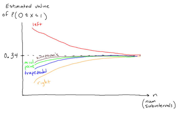
PART 2
Location: assignment-problems
Skim the following section of http://learnyouahaskell.com/starting-out.
Texas ranges I'm a list comprehension
Create Haskell file ComplicatedList.hs and write a function calcList in that takes an input number n and counts the number of ordered pairs [x,y] that satisfy $-n \leq x,y \leq n$ and $x-y \leq \dfrac{xy}{2} \leq x+y$ and $x,y \notin \{ -2, -1, 0, 1, 2 \}.$ This function should generate a list comprehension and then count the length of that list.
To check your function, print calcList 50. You should get a result of $16.$
PART 3
Complete these C++/Shell/SQL coding challenges and submit screenshots.
https://www.hackerrank.com/challenges/c-tutorial-for-loop/problem
https://www.hackerrank.com/challenges/c-tutorial-functions/problem
https://www.hackerrank.com/challenges/bash-tutorials---comparing-numbers/problem
https://www.hackerrank.com/challenges/bash-tutorials---more-on-conditionals/problem
https://sqlzoo.net/wiki/SELECT_within_SELECT_Tutorial (queries 4,5,6)
For C++/Shell, each screenshot should include your username, the problem title, and the "Status: Accepted" indicator.
For SQL, each screenshot should include the problem number, the successful smiley face, and your query.
Here's a helpful example of some bash syntax. (The spaces on the inside of the brackets are really important! It won't work if you remove the spaces, i.e.
[$n -gt 100])read n if [ $n -gt 100 ] || [ $n -lt -100 ] then echo What a large number. else echo The number is smol. if [ $n -eq 13 ] then echo And it\'s unlucky!!! fi fi
PART 4
a.
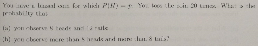
b.
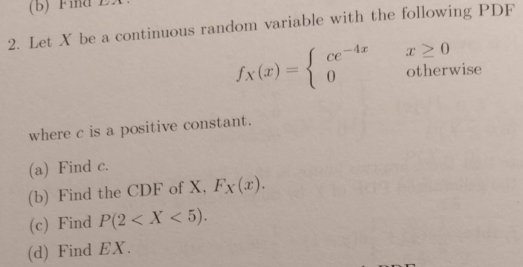
Remember that for a probability distribution $f(x),$ the cumulative distribution function (CDF) is $F(x) = P(X \leq x) = \displaystyle \int_{-\infty}^x f(x) \, \textrm dx.$
Remember that $EX$ means $\textrm E[X].$
Problem 78-3
Review; 10% of assignment grade; 15 minutes estimate
Commit your code to GitHub. When you submit your assignment, include a link to your commit(s). If you don't do this, your assignment will receive a grade of $0$ until you resubmit with links to your commits.
Additionally, do the following:
Make 2 GitHub issues on your assigned classmate's repository (but NOT
assignment-problems). See eurisko.us/resources/#code-reviews to determine your assigned classmate. When you submit your assignment, include the links to the issues you created.~Resolve an issue that has been made on your own GitHub repository. When you submit your assignment, include a link to the issue you resolved. (If you don't have any issues on any of your repositories, then you don't have to do anything, but state that this is the case when you turn in your assignment.)~ Let's actually hold off on this bit for the next couple weeks, so that we can build up an inventory of issues on our repositories. Then, once we have an inventory of 5-10 issues to choose from each time, we can start resolving them.
SUBMISSION TEMPLATE
For your submission, copy and paste your links into the following template:
Commit link to machine-learning repo (if any changes were required): _____

Repl.it link to Haskell code: _____
Commit link for assignment-problems repo: _____

Link to C++/SQL screenshots (Overleaf or Google Doc): _____
Link to probability solutions (on Overleaf):

Issue 1: _____
Issue 2: _____
Problem 77-1
Primary problems; 45% of assignment grade; 75 minutes estimate
a. You'll need to do part 1 of the supplemental problem before you do this problem.
(i) Download the freshman_lbs.csv dataset from https://people.sc.fsu.edu/~jburkardt/data/csv/csv.html, read it into a DataFrame, and create 5 test-train splits:
- Testing data = first 20% of the records, training data = remaining 80%
- Testing data = second 20% of the records, training data = remaining 80%
- Testing data = third 20% of the records, training data = remaining 80%
- Testing data = fourth 20% of the records, training data = remaining 80%
- Testing data = fifth 20% of the records, training data = remaining 80%
Note that you'll need to convert the appropriate entries to numbers (instead of strings) in the dataset. There are 2 options for doing this:
Option 1: don't worry about fixing the format within the
read_csvmethod. Just do something likedf = df.apply('weight', lambda x: int(x))afterwards, before you pass the dataframe into your model.Option 2: when you read in the csv, after you do the
lines = file.read().split('\n')
entries = [line.split(',') for line in lines]
thing, you can loop through the entries, and if
entry[0]+entry[-1] == '""', then you can setentry = entry[1:-1]to remove the quotes. Otherwise, ifentry[0]+entry[-1] != '""', then you can try to doentry = float(entry[1:-1]).
(ii) For each test-train split, fit each of the following models on the training data and use it to predict the sexes on the testing data. (You are predicting sex as a function of weight and BMI, and you can just use columns corresponding to September data.)
Decision tree using Gini split criterion
A single random decision tree
Random forest with 10 trees
Random forest with 100 trees
Random forest with 1000 trees
(iii) For each model, compute the accuracy (count the total number of correct classifications and divide by the total number of classifications). Put these results in a table in an Overleaf document.
Note that the total number of classifications should be equal to the total number of records in the dataset (you did 5 train-test splits, and each train-test split involved testing on 20% of the data).
(iv) Below the table, analyze the results. Did you expect these results, or did they surprise you? Why do you think you got the results you did?
b. For each of your classmates, copy over their DumbStrategy and CombatStrategy and run your DumbPlayer/CombatPlayer tests using your classmate's strategy. Fill out the following information for each classmate:
Name of classmate
When you copied over their
DumbStrategyand ran your DumbPlayer tests, did they pass? If not, then what's the issue? Is it a problem with your game, or with their strategy class?When you copied over their
CombatStrategyand ran your CombatPlayer tests, did they pass? If not, then what's the issue? Is it a problem with your game, or with their strategy class?
Problem 77-2
Supplemental problems; 45% of assignment grade; 75 minutes estimate
PART 1
In your machine-learning repository, create a folder machine-learning/datasets/. Go to https://people.sc.fsu.edu/~jburkardt/data/csv/csv.html, download the file airtravel.csv, and put it in your datasets/ folder.
In Python, you can read a csv as follows:
>>> path_to_datasets = '/home/runner/machine-learning/datasets/'
>>> filename = 'airtravel.csv'
>>> with open(path_to_datasets + filename, "r") as file:
   print(file.read())

"Month", "1958", "1959", "1960"
"JAN",  340,  360,  417
"FEB",  318,  342,  391
"MAR",  362,  406,  419
"APR",  348,  396,  461
"MAY",  363,  420,  472
"JUN",  435,  472,  535
"JUL",  491,  548,  622
"AUG",  505,  559,  606
"SEP",  404,  463,  508
"OCT",  359,  407,  461
"NOV",  310,  362,  390
"DEC",  337,  405,  432
Write a @classmethod called DataFrame.from_csv(path_to_csv, header=True) that constructs a DataFrame from a csv file (similar to how DataFrame.from_array(arr) constructs the DataFrame from an array).
Test your method as follows:
>>> path_to_datasets = '/home/runner/machine-learning/datasets/'
>>> filename = 'airtravel.csv'
>>> filepath = path_to_datasets + filename
>>> df = DataFrame.from_csv(filepath, header=True)

>>> df.to_array()
[['"Month"', '"1958"', '"1959"', '"1960"'],
['"JAN"',  '340',  '360',  '417'],
['"FEB"',  '318',  '342',  '391'],
['"MAR"',  '362',  '406',  '419'],
['"APR"',  '348',  '396',  '461'],
['"MAY"',  '363',  '420',  '472'],
['"JUN"',  '435',  '472',  '535'],
['"JUL"',  '491',  '548',  '622'],
['"AUG"',  '505',  '559',  '606'],
['"SEP"',  '404',  '463',  '508'],
['"OCT"',  '359',  '407',  '461'],
['"NOV"',  '310',  '362',  '390'],
['"DEC"',  '337',  '405',  '432']]
PART 2
Location: assignment-problems
Skim the following section of http://learnyouahaskell.com/starting-out.
An intro to lists
Create Haskell file ListProcessing.hs and write a function prodFirstLast in Haskell that takes an input list arr and computes the product of the first and last elements of the list. Then, apply this function to the input [4,2,8,5].
Tip: use the !! operator and the length function.
Your file will look like this:
prodFirstLast arr = (your code here)
main = print (prodFirstLast [4,2,8,5])
Note that, to print out an integer, we use print instead of putStrLn.
(You can also use print for most strings. The difference is that putStrLn can show non-ASCII characters like "я" whereas print cannot.)
Run your function and make sure it gives the desired output (which is 20).
PART 3
a. Complete these introductory C++ coding challenges and submit screenshots:
https://www.hackerrank.com/challenges/c-tutorial-basic-data-types/problem
https://www.hackerrank.com/challenges/c-tutorial-conditional-if-else/problem
b. Complete these Bash coding challenges and submit screenshots:
https://www.hackerrank.com/challenges/bash-tutorials---a-personalized-echo/problem
https://www.hackerrank.com/challenges/bash-tutorials---the-world-of-numbers/problem
(Each screenshot should include your username, the problem title, and the "Status: Accepted" indicator.)
c. Complete SQL queries 1-3 here and submit screenshots:
(Each screenshot should include the problem number, the successful smiley face, and your query.)
PART 4
a. As we will see in the near future, the standard normal distribution comes up A LOT in the context of statistics. It is defined as
$$ p(x) = \dfrac{1}{\sqrt{2\pi}} e^{-x^2/2}. $$The reason why we haven't encountered it until now is that it's difficult to integrate. In practice, it's common to use a pre-computed table of values to look up probabilities from this distribution.
The actual problem: Write a function calc_standard_normal_probability(a,b) to approximate $P(a \leq X \leq b)$ for the standard normal distribution, using a Riemann sum with step size 0.001.
To check your function, print out estimates of the following probabilities:
$P(-1 \leq x \leq 1)$
$P(-2 \leq x \leq 2)$
$P(-3 \leq x \leq 3)$
Your estimates should come out close to 0.68, 0.955, 0.997 respectively. (https://en.wikipedia.org/wiki/68%E2%80%9395%E2%80%9399.7_rule)
b.
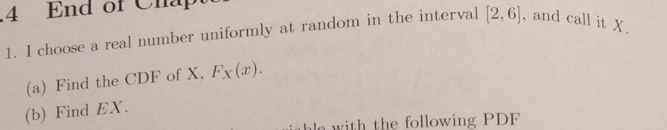
"CDF" stands for Cumulative Distribution Function. The CDF of a probability distribution $f(x)$ is defined as $$ F(x) = P(X \leq x) = \int_{-\infty}^x f(x) \, \textrm dx. $$
Your answer for the CDF will be a piecewise function (3 pieces).
$EX$ means $E[X].$
c.

Problem 77-3
Review; 10% of assignment grade; 15 minutes estimate
Commit your code to GitHub. When you submit your assignment, include a link to your commit(s). If you don't do this, your assignment will receive a grade of $0$ until you resubmit with links to your commits.
Additionally, do the following:
Make 2 GitHub issues on your assigned classmate's repository (but NOT
assignment-problems). See eurisko.us/resources/#code-reviews to determine your assigned classmate. When you submit your assignment, include the links to the issues you created.~Resolve an issue that has been made on your own GitHub repository. When you submit your assignment, include a link to the issue you resolved. (If you don't have any issues on any of your repositories, then you don't have to do anything, but state that this is the case when you turn in your assignment.)~ Let's actually hold off on this bit for the next couple weeks, so that we can build up an inventory of issues on our repositories. Then, once we have an inventory of 5-10 issues to choose from each time, we can start resolving them.
Problem 76-1
Primary problems; 40% of assignment grade; 60 minutes estimate
a. Create a RandomForest class in machine-learning/src/random-forest that is initialized with a value n that represents the number of random decision trees to use.
The RandomForest should have a fit() method and a predict() method, just like the DecisionTree.
The
fit()method should fit all the random decision trees.The
predict()method should get a prediction from each random decision tree, and then return the prediction that occurred most frequently. (If there are multiple predictions that occurred most frequently, then choose randomly among them.)
So it should work like this:
rf = RandomForest(10) # random forest consisting of 10 random trees
rf.fit(df) # fit all 10 of those trees to the dataframe
rf.predict(observation) # have each of the 10 trees make a prediction, and
                        # return the majority vote of the 10 trees
b. Refactor the combat_state in your game.
Previously, it looked like this:
[
    {'location': (1,2),
    'order': [{'player': 1, 'unit': 0,},
              {'player': 0, 'unit': 1},
              {'player': 1, 'unit': 1}]
    },
    {'location': (5,10),
    'order': [{'player': 0, 'unit': 0},
              {'player': 1, 'unit': 2},
              {'player': 1, 'unit': 4}]
    }
]
Now, we will refactor the above into this:
{
    (1,2): [{'player': 1, 'unit': 0},
            {'player': 0, 'unit': 1},
            {'player': 1, 'unit': 1},
            {'player': 1, 'unit': 2}]
    (2,2): [{'player': 2, 'unit': 0},
            {'player': 3, 'unit': 1},
            {'player': 2, 'unit': 1},
            {'player': 2, 'unit': 2}]
}
As a result, we will also have to update the inputs to decide_which_unit_to_attack. Originally, the inputs were as follows:
decide_which_unit_to_attack(self, combat_state, attacker_index)Now, we will have to include an additional input location as follows:
decide_which_unit_to_attack(self, combat_state, location, attacker_index)c. Refactor your decide_removals function into a function decide_removal (singular, not plural) that returns the index of a single ship to remove. So, it will return a single integer instead of an array.
Then, refactor your game so that it calls decide_removal repeatedly until no more removals are required. This will prevent a situation in which our game crashes because a player did not remove enough ships.
def decide_removal(self, game_state):
        ...
        return the unit index of the ship that you want to remove.

        for example, if you want to remove the unit at index 2,
        return 2
Problem 76-2
Supplemental problems; 50% of assignment grade; 75 minutes estimate
PART 1
Location: assignment-problems
Write a function random_draw(distribution) that draws a random number from the probability distribution. Assume that the distribution is an array such that distribution[i] represents the probability of drawing i.
Here are some examples:
random_draw([0.5, 0.5])will return0or1with equal probabilityrandom_draw([0.25, 0.25, 0.5])will return0a quarter of the time,1a quarter of the time, and2half of the timerandom_draw([0.05, 0.2, 0.15, 0.3, 0.1, 0.2])will return05% of the time,120% of the time,215% of the time,330% of the time,410% of the time, and0.220% of the time.
The way to implement this is to
- turn the distribution into a cumulative distribution,
- choose a random number between 0 and 1, and then
- find the index of the first value in the cumulative distribution that is greater than the random number.
Distribution:
    [0.05, 0.2, 0.15, 0.3, 0.1, 0.2]

Cumulative distribution:
    [0.05, 0.25, 0.4, 0.7, 0.8, 1.0]

Choose a random number between 0 and 1:
    0.77431

The first value in the cumulative distribution that is
greater than 0.77431 is 0.8.

This corresponds to the index 4.

So, return 4.
To test your function, generate 1000 random numbers from each distribution and ensure that their average is close to the true expected value of the distribution.
In other words, for each of the following distributions, print out the true expected value, and then print out the average of 1000 random samples.
[0.5, 0.5][0.25, 0.25, 0.5][0.05, 0.2, 0.15, 0.3, 0.1, 0.2]
PART 2
Location: assignment-problems
Skim the following sections of http://learnyouahaskell.com/starting-out.
- Ready, set, go!
- Baby's first functions
Create Haskell file ClassifyNumber.hs and write a function classifyNumber in Haskell that takes an input number x and returns
"negative"ifxis negative"nonnegative"ifxis nonnegative.
Then, apply this function to the input 5.
Your file will look like this:
classifyNumber x = (your code here)
main = putStrLn (classifyNumber 5)
Now, run your function by typing the following into the command line:
>>> ghc --make ClassifyNumber
>>> ./ClassifyNumber
ghc is a Haskell compiler. It will compile or "make" an executable object using your .hs file. The command ./ClassifyNumber. actually runs your executable object.
PART 3
Complete this introductory C++ coding challenge: https://www.hackerrank.com/challenges/cpp-input-and-output/problem
Submit a screenshot that includes the name of the problem (top left), your username (top right), and Status: Accepted (bottom).

PART 4
Complete this introductory Shell coding challenge: https://www.hackerrank.com/challenges/bash-tutorials---looping-and-skipping/problem
The following example of a for loop will be helpful:
for i in {2..10}
do
    ((n = 5 * i))
    echo $n
doneNote: You can solve this problem with just a single for loop
Again, submit a screenshot that includes the name of the problem (top left), your username (top right), and Status: Accepted (bottom), just like in part 3.
PART 5
Complete queries 11-14 here: https://sqlzoo.net/wiki/SELECT_from_Nobel_Tutorial
As usual, include a screenshot for each problem that includes the problem number, the successful smiley face, and your query.
PART 6
Location: Overleaf
Complete the following probability problems:
a.
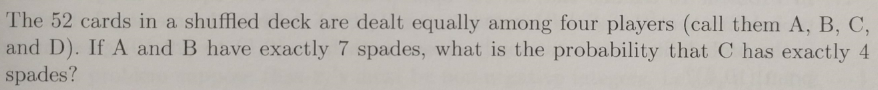
- Use conditional probability. In other words, compute the probability that C has exactly $4$ spaces, given that A and B have exactly 7 spaces (together).
b.
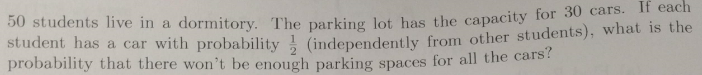
- Write your answer using sigma notation or "dot dot dot" notation.
Problem 76-3
Review; 10% of assignment grade; 15 minutes estimate
Commit your code to GitHub. When you submit your assignment, include a link to your commit(s). If you don't do this, your assignment will receive a grade of $0$ until you resubmit with links to your commits.
Additionally, do the following:
Make a GitHub issue on your assigned classmate's repository (but NOT
assignment-problems). See eurisko.us/resources/#code-reviews to determine your assigned classmate. When you submit your assignment, include a link to the issue you created.Resolve an issue that has been made on your own GitHub repository. When you submit your assignment, include a link to the issue you resolved. (If you don't have any issues on any of your repositories, then you don't have to do anything, but state that this is the case when you turn in your assignment.)
Problem 75-1
Location: machine-learning/src/decision_tree.py
Grade Weighting: 40%
Update your DecisionTree to have the option to build the tree via random splits. By "random splits", I mean that the tree should randomly choose from the possible splits, and it should keep splitting until each leaf node is pure.
>>> dt = DecisionTree(split_metric = 'gini')
>>> dt.fit(df)
Fits the decision tree using the Gini metric

>>> dt = DecisionTree(split_metric = 'random')
>>> dt.fit(df)
Fits the decision tree by randomly choosing splits
Problem 75-2
Estimated Time: 60 minutes
Grade Weighting: 40%
Submit corrections to final (put your corrections in an overleaf doc). I made a final review video that goes through each problem, available here: https://vimeo.com/496684498
For each correction, explain
- what misunderstanding you had, and
- how you get to the correct result.
Important: The majority of the misunderstandings should NOT be "I ran out of time", and when you explainhow to get to the correct result, SHOW ALL WORK.
Problem 75-3
Grade Weighting: 20%
Make sure that problem 73-1 is done. In the next assignment, you will run everyone else's strategies and they will run yours as well. We should all get the same results.
Problem 75-4
Estimated Time: 20 minutes
Important! If you don't do the things below, your assignment will receive a grade of zero.
Commit your code to GitHub. When you submit your assignment, include a link to your commit(s).
Make a GitHub issue on your assigned classmate's repository (but NOT
assignment-problems). See eurisko.us/resources/#code-reviews to determine your assigned classmate. When you submit your assignment, include a link to the issue you created.Resolve an issue that has been made on your own GitHub repository. When you submit your assignment, include a link to the issue you resolved.
Problem 74-1
Wrapping up the semester...
Read the edited version of your blog post here. If you'd like to see any changes, post on Slack by the end of the week. Otherwise, these are going up on the website!
Turn in any missing assignments / resubmissions / reviews / test corrections by Sunday 1/3 at the very latest. Finish strong! I want to give out strong grades, but I can only do that if you're up to date with all your work and you've done it well.
Problem 74-2
Study for the final!
Probability/Statistics
definitions of independent/disjoint, conditional probability, mean, variance, standard deviation, covariance, how variance/covariance are related to expectation identifying probability distributions, solving for an unknown constant so that a probability distribution is valid, discrete uniform, continuous uniform, exponential, poisson, using cumulative distributions i.e. P(a <= x < b) = P(x < b) - P(x < a), KL divergence, joint distributions, basic probability computations with joint distributions, likelihood distribution, posterior/prior distributions
Machine Learning
pseudoinverse, fitting a linear regression, fitting a logistic regression, end behaviors of linear and logistic regression, interaction terms, using linear regression to fit the coefficients of a nonlinear function, categorical variables, naive bayes, k-nearest neighbors, decision trees, leave-one-out cross validation, underfitting/overfitting, training/testing datasets (testing datasets are also known as validation datasets)
Algorithms
Intelligent search (backtracking), depth-first search, breadth-first search, shortest path in a graph using breadth-first search, quicksort, computing big-O notation given a recurrence, bisection search (also known as bisection search)
Simulation
euler estimation, SIR model, predator-prey model, hodgkin-huxley model, translating a description into a system of differential equations
Review
Basic string processing (something like separate_into_words and reverse_word_order from Quiz 1), Implementing a recursive sequence, unlisting, big-O notation, matrix multiplication, converting to reduced row echelon form, determinant using rref, determinant using cofactors, why determinant using rref is faster than determinant using cofactors, inverse via augmented matrix, tally sort, merge sort (also know how to merge two sorted lists), swap sort, Newton-Raphson (i.e. the “zero of tangent line” method), gradient descent, grid search (also know how to compute cartesian product), Linked list, tree, stack, queue, converting between binary and decimal
Problem 73-1
Estimated Time: 2 hours
Points: 20
Refactor your game so that strategies adhere to this format exactly. Put the strategies as separate files in src/strategies.
Note: If you have any disagreements with the strategy template below, post on Slack, and we can discuss.
from units.base import Base
from units.battlecruiser import Battlecruiser
from units.battleship import Battleship
from units.colony import Colony
from units.cruiser import Cruiser
from units.destroyer import Destroyer
from units.dreadnaught import Dreadnaught
from units.scout import Scout
from units.shipyard import Shipyard

class CombatStrategy:

    def __init__(self, player_index):
        self.player_index = player_index

    def will_colonize_planet(self, coordinates, game_state):
        ...
        return either True or False

    def decide_ship_movement(self, unit_index, game_state):
        ...
        return a "translation" which is a tuple representing
        the direction in which the ship moves.

        # For example, if a unit located at (1,2) wanted to
        # move to (1,1), then the translation would be (0,-1).

    def decide_purchases(self, game_state):
        ...
        return {
            'units': list of unit objects you want to buy,
            'technology': list of technology attributes you want to upgrade
        }

        # for example, if you wanted to buy 2 Scouts, 1 Destroyer,
        # upgrade defense technology once, and upgrade attack
        # technology twice, you'd return
        # {
        #     'units': [Scout, Scout, Destroyer],
        #     'technology': ['defense', 'attack', 'attack']
        # }

    def decide_removals(self, game_state):
        ...
        return a list of unit indices of ships that you want to remove.

        # for example, if you want to remove your 0th and 3rd units, you'd
        # return [0, 3]

    def decide_which_unit_to_attack(self, combat_state, attacker_index):

        # combat_state is the combat_state for the particular battle
        # being considered. It will take the form
        # {'location': (1,2),
        #     'order': [{'player': 1, 'unit': 0},
        #               {'player': 0, 'unit': 1},
        #               {'player': 1, 'unit': 1},
        #               {'player': 1, 'unit': 2}],
        # }.

        # attacker_index is the index of your unit, whose turn it is
        # to attack.

        ...

        return the index of the ship you want to attack in the
        combat order.

        # in the above example, if you want to attack player 1's unit 1,
        # then you'd return 2 because it corresponds to
        # combat_state['order'][2]

    def decide_which_units_to_screen(self, combat_state):

        # again, the combat_state is the combat_state for the
        # particular battle

        ...

        return the indices of the ships you want to screen
        in the combat order

        # in the above example, if you are player 1 and you want
        # to screen units 1 and 2, you'd return [2,3] because
        # the ships you want to screen are
        # combat_state['order'][2] and combat_state['order'][3]

        # NOTE: FOR COMBATSTRATEGY AND DUMBSTRATEGY,
        # YOU CAN JUST RETURN AN EMPTY ARRAY
Note: for technology upgrades, you'll likely have to translate between strings of technology names and technology stored as Player attributes. The setattr and getattr functions may be helpful:
>>> class Cls:
        pass
>>> obj = Cls()
>>> setattr(obj, "foo", "bar")
>>> obj.foo
'bar'
>>> getattr(obj, "foo")
'bar'
Problem 73-2
Estimated Time: 1 hour
Points: 15
We need to extend our EulerEstimator to allow for "time delay". To do this, we'll need to keep a cache of data for the necessary variables. However, it's going to be very hard to build this if we always have to refer to variables by their index in the point. So, in this problem, we're going to update our EulerEstimator so that we can refer to variables by their actual names.
Refactor your EulerEstimator so that x is a dictionary instead of an array. This way, we can reference components of x by their actual labels rather than having to always use indices.
For example, to run our SIR model, we originally did this:
derivatives = [
    (lambda t, x: -0.0003*x[0]*x[1]),
    (lambda t, x: 0.0003*x[0]*x[1] - 0.02*x[1]),
    (lambda t, x: 0.02*x[1])
]
starting_point = (0, (1000, 1, 0))

estimator = EulerEstimator(derivatives, starting_point)
Now, we need to refactor it into this:
derivatives = {
    'susceptible': (lambda t, x: -0.0003*x['susceptible']*x['infected']),
    'infected': (lambda t, x: 0.0003*x['susceptible']*x['infected'] - 0.02*x['infected']),
    'recovered': (lambda t, x: 0.02*x['infected'])
}
starting_point = (0, {'susceptible': 1000, 'infected': 1, 'recovered': 0})

estimator = EulerEstimator(derivatives, starting_point)
Update the code in test_euler_estimator.py and 3_neuron_network.py to adhere to this new convention.
When I check your submission, I'm going to check that your EulerEstimator has been initialized with a dictionary in each of these files, and I'm going to run each of these files to make sure that they generate the same plots as before.
Problem 72-1
Estimated Time: 15 minutes
Location:
machine-learning/analysis/scatter_plot.py
Points: 5
Make a scatter plot of the following dataset consisting of the points (x, y, class). When the class is A, color the dot red. When it is B, color the dot blue. Post your plot on slack once you've got it.
data = [[2,13,'B'],[2,13,'B'],[2,13,'B'],[2,13,'B'],[2,13,'B'],[2,13,'B'],
    [3,13,'B'],[3,13,'B'],[3,13,'B'],[3,13,'B'],[3,13,'B'],[3,13,'B'],
    [2,12,'B'],[2,12,'B'],
    [3,12,'A'],[3,12,'A'],
    [3,11,'A'],[3,11,'A'],
    [3,11.5,'A'],[3,11.5,'A'],
    [4,11,'A'],[4,11,'A'],
    [4,11.5,'A'],[4,11.5,'A'],
    [2,10.5,'A'],[2,10.5,'A'],
    [3,10.5,'B'],
    [4,10.5,'A']]
In the plot, make the dot size proportional to the number of points at that location.
For example, to plot a data set
[
 (1,1),
 (2,4), (2,4),
 (3,9), (3,9), (3,9), (3,9),
 (4,16), (4,16), (4,16), (4,16), (4,16), (4,16), (4,16), (4,16), (4,16)
 ]
you would use the following code:
import matplotlib.pyplot as plt
plt.scatter(x=[1, 2, 3, 4], y=[1, 4, 9, 16], s=[20, 40, 80, 160], c='red')

Problem 72-2
Estimated Time: 10-60 minutes (depending on whether you've got bugs)
Location:
machine-learning/src/decision_tree.py
machine-learning/tests/test_decision_tree.py
Points: 10
Refactor your DecisionTree so that the dataframe is passed in the fit method (not when the decision tree is initialized). Also, create a method to classify points.
Then, make sure decision tree passes the following tests, using the data from problem 71-1.
Note: Based on visually inspecting a plot of the data, I think these tests are correct, but if you get something different (that looks reasonable), post on Slack so I can check.
df = DataFrame.from_array(data, columns = ['x', 'y', 'class'])

>>> dt = DecisionTree()
>>> dt.fit(df)

The tree should look like this:

                           (13A, 15B)
                            /      \
                  (y < 12.5)       (y >= 12.5)
                  (13A, 3B)        (12B)
                  /         \
          (x < 2.5)          (x >= 2.5)
          (2A, 2B)                (11A, 1B)
         /     \                  /        \
(y < 11.25)   (y >= 11.25)  (y < 10.75)     (y >= 10.75)
(2A)          (2B)          (1A, 1B)        (10A)
                            /      \
                   (x < 3.5)        (x >= 3.5)
                        (1B)        (1A)

>>> dt.root.best_split
('y', 12.5)
>>> dt.root.low.best_split
('x', 2.5)
>>> dt.root.low.low.best_split
('y', 11.25)
>>> dt.root.low.high.best_split
('y', 10.75)
>>> dt.root.low.high.low.best_split
('x', 3.5)

>>> dt.classify({'x': 2, 'y': 11.5})
'B'
>>> dt.classify({'x': 2.5, 'y': 13})
'B'
>>> dt.classify({'x': 4, 'y': 12})
'A'
>>> dt.classify({'x': 3.25, 'y': 10.5})
'B'
>>> dt.classify({'x': 3.75, 'y': 10.5})
'A'
Problem 72-3
Estimated time: 45 minutes
Location: Overleaf
Grading: 5 points
a.
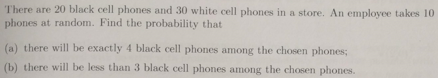
b.
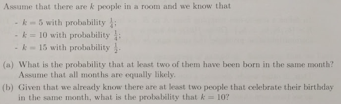
- For part (a), you need to compute the probability of each "path" to the desired outcome:
- For part (b), start with $P(\text{k=10} \, | \, \text{2 born in same month} ),$ and use the following two equivalent statements of Bayes' theorem:
Problem 72-4
Estimated time: 45 minutes
Location: Overleaf
Grading: 5 points
- Complete queries 1-10 in SQL Zoo Module 3. Take a screenshot of each successful query (with the successful smiley face showing) and put them in the overleaf doc.
Problem 71-1
Estimated Time: 45 minutes
Location:
machine-learning/src/decision_tree.py
machine-learning/tests/test_decision_tree.py
Points: 15
If you haven't already, create a split() method in your DecisionTree (not the same as the split() method in your Node!) that splits the tree at the node with highest impurity.
Then, create a fit() method in your DecisionTree that keeps on split()-ing until all terminal nodes are completely pure.
Assert that the following tests pass:
>>> df = DataFrame.from_array(
    [[1, 11, 'A'],
    [1, 12, 'A'],
    [2, 11, 'A'],
    [1, 13, 'B'],
    [2, 13, 'B'],
    [3, 13, 'B'],
    [3, 11, 'B']],
    columns = ['x', 'y', 'class']
)
>>> dt = DecisionTree(df)

# currently, the decision tree looks like this:

                      (3A, 4B)

>>> dt.split()
# now, the decision tree looks like this:

                      (3A, 4B)
                      /      \
            (y < 12.5)       (y >= 12.5)
            (3A, 1B)         (3B)

>>> dt.split()
# now, the decision tree looks like this:

                    (3A, 4B)
                    /      \
           (y < 12.5)       (y >= 12.5)
           (3A, 1B)         (3B)
         /         \
(x < 2.5)          (x >= 2.5)
(3A)               (1B)

>>> dt.root.high.row_indices
[3, 4, 5]
>>> dt.root.low.low.row_indices
[0, 1, 2]
>>> dt.root.low.high.row_indices
[6]

>>> dt = DecisionTree(df)

# currently, the decision tree looks like this:

                      (3A, 4B)

>>> dt.fit()
# now, the decision tree looks like this:

                    (3A, 4B)
                    /      \
           (y < 12.5)       (y >= 12.5)
           (3A, 1B)         (3B)
         /         \
(x < 2.5)          (x >= 2.5)
(3A)               (1B)

>>> dt.root.high.row_indices
[3, 4, 5]
>>> dt.root.low.low.row_indices
[0, 1, 2]
>>> dt.root.low.high.row_indices
[6]
Problem 71-2
Estimated time: 45 minutes
Location: Overleaf
Grading: 10 points
- Complete queries 6-13 in SQL Zoo Module 2. Take a screenshot of each successful query (with the successful smiley face showing) and put them in the overleaf doc.
Problem 71-3
Estimated time: 45 minutes
Location: Overleaf
Grading: 10 points
(Taken from Introduction to Probability: Statistics and Random Processes by Hossein Pishro-Nik)
a.
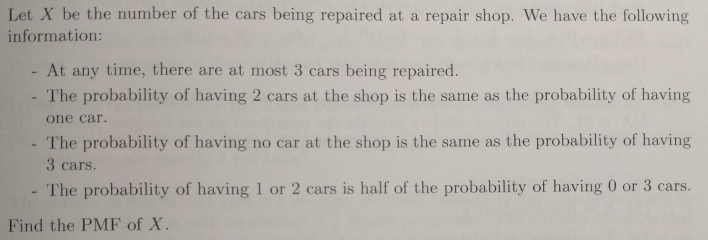
b.
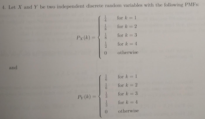
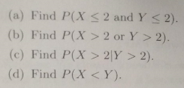
c.

Problem 70-1
Estimated time: 60 min
Grading: 10 points
Locations:
machine-learning/src/leave_one_out_cross_validator.py
machine-learning/tests/test_leave_one_out_cross_validator.py
Write a class LeaveOneOutCrossValidator that computes percent_accuracy (also known as "leave-one-out cross validation") for any input classifier. For a refresher, see problem 58-1.
Assert that LeaveOneOutCrossValidator passes the following tests:
>>> df = the cookie dataset that's in test_k_nearest_neighbors_classifier.py
>>> knn = KNearestNeighborsClassifier(k=5)

>>> cv = LeaveOneOutCrossValidator(knn, df, prediction_column='Cookie Type')
    [ Note: under the hood, the LeaveOneOutCrossValidator should
      create a leave_one_out_df and do
      knn.fit(leave_one_out_df, prediction_column='Cookie Type') ]

>>> cv.accuracy()
0.7894736842105263 (Updated!)

Note: the following is included to help you debug.
Row 0 -- True Class is Shortbread; Predicted Class was Shortbread
Row 1 -- True Class is Shortbread; Predicted Class was Shortbread
Row 2 -- True Class is Shortbread; Predicted Class was Shortbread
Row 3 -- True Class is Shortbread; Predicted Class was Shortbread
Row 4 -- True Class is Sugar; Predicted Class was Sugar
Row 5 -- True Class is Sugar; Predicted Class was Sugar
Row 6 -- True Class is Sugar; Predicted Class was Sugar
Row 7 -- True Class is Sugar; Predicted Class was Shortbread
Row 8 -- True Class is Sugar; Predicted Class was Shortbread
Row 9 -- True Class is Sugar; Predicted Class was Sugar
Row 10 -- True Class is Fortune; Predicted Class was Fortune (Updated!)
Row 11 -- True Class is Fortune; Predicted Class was Fortune
Row 12 -- True Class is Fortune; Predicted Class was Fortune
Row 13 -- True Class is Fortune; Predicted Class was Shortbread
Row 14 -- True Class is Fortune; Predicted Class was Fortune (Updated!)
Row 15 -- True Class is Shortbread; Predicted Class was Sugar
Row 16 -- True Class is Shortbread; Predicted Class was Shortbread
Row 17 -- True Class is Shortbread; Predicted Class was Shortbread
Row 18 -- True Class is Shortbread; Predicted Class was Shortbread

>>> accuracies = []
>>> for k in range(1, len(data)-1):
>>>    knn = KNearestNeighborsClassifier(k)
>>>    cv = LeaveOneOutCrossValidator(knn, df, prediction_column='Cookie Type')
>>>    accuracies.append(cv.accuracy())

>>> accuracies
 [0.5789473684210527,
 0.5789473684210527, #(Updated!)
 0.5789473684210527,
 0.5789473684210527,
 0.7894736842105263, #(Updated!)
 0.6842105263157895,
 0.5789473684210527,
 0.5789473684210527, #(Updated!)
 0.6842105263157895, #(Updated!)
 0.5263157894736842,
 0.47368421052631576, #(Updated!)
 0.42105263157894735,
 0.42105263157894735, #(Updated!)
 0.3684210526315789, #(Updated!)
 0.3684210526315789, #(Updated!)
 0.3684210526315789, #(Updated!)
 0.42105263157894735]
Problem 70-2
Estimated time: 45 minutes
Grading: 10 points
Location: Overleaf
Suppose you are a mission control analyst who is looking down at an enemy headquarters through a satellite view, and you want to get an estimate of how many tanks they have. Most of the headquarters is hidden, but you notice that near the entrance, there are four tanks visible, and these tanks are labeled with the numbers $52, 30, 68, 7.$ So, you assume that they have $N$ tanks that they have labeled with numbers from $1$ to $N.$
Your commander asks you for an estimate: with $95\%$ certainty, what's the max number of tanks they have? Be sure to show your work.
In this problem, you'll answer that question using the same process that you used in Problem 41-1. See here for some additional clarifications that were added to this problem when it was given to the Computation & Modeling class.

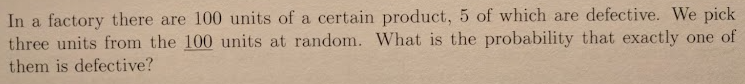
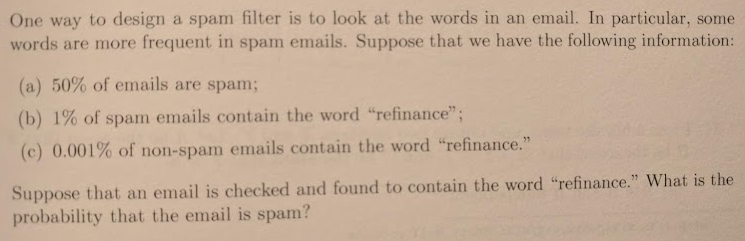
Problem 69-1
Grading: 10 points
George & David, this will be a catch-up problem for you guys. You guys are missing a handful of recent assignments, and there are some key problems that serve as foundations for future problems. These are the key problems: 67-1, 66-1, 62-1 (in that order of importance).
- Your task for this assignment is to complete and submit those problems.
Colby, this is also a catch-up problem for you -- your task is to complete 68-1.
Eli & Riley you'll get 10 points for this problem because you're up-to-date.
Problem 69-2
Grading: extra credit (you can get 200% on this assignment)
Location: assignment-problems/sudoku_solver.py
Use "intelligent search" to solve the following mini sudoku puzzle. Fill in the grid so that every row, every column, and every 3x2 box contains the digits 1 through 6.
For a refresher on "intelligent search", see problem 44-1.
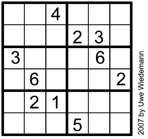
Format your output so that when your code prints out the result, it prints out the result in the shape of a sudoku puzzle:
-----------------
| . . 4 | . . . |
| . . . | 2 3 . |
-----------------
| 3 . . | . 6 . |
| . 6 . | . . 2 |
-----------------
| . 2 1 | . . . |
| . . . | 5 . . |
-----------------
Problem 68-1
Estimated Time: 2-3 hours
Location:
machine-learning/src/decision_tree.py
machine-learning/tests/test_decision_tree.py
Points: 15
In this problem, you will create the first iteration of a class DecisionTree that builds a decision tree by repeatedly looping through all possible splits and choosing the split with the highest "goodness of split".
We will use the following simple dataset:
['x', 'y', 'class']
[1, 11, 'A']
[1, 12, 'A']
[2, 11, 'A']
[1, 13, 'B']
[2, 13, 'B']
[3, 12, 'B']
[3, 13, 'B']
For this dataset, "all possible splits" mean all midpoints between distinct entries in sorted data columns.
The sorted distinct entries of
xare 1, 2, 3.The sorted distinct entries of
yare 11, 12, 13.
So, "all possible splits" are x=1.5, x=2.5, y=11.5, y=12.5.
Assert that the following tests pass. Note that you will need to create a Node class for the nodes in your decision tree.
>>> df = DataFrame.from_array(
    [[1, 11, 'A'],
    [1, 12, 'A'],
    [2, 11, 'A'],
    [1, 13, 'B'],
    [2, 13, 'B'],
    [3, 13, 'B'],
    [3, 11, 'B']],
    columns = ['x', 'y', 'class']
)
>>> dt = DecisionTree(df)

>>> dt.root.row_indices
[0, 1, 2, 3, 4, 5, 6] # these are the indices of data points in the root node

>>> dt.root.class_counts
{
    'A': 3,
    'B': 4
}

>>> dt.root.impurity
0.490 # rounded to 3 decimal places

>>> dt.root.possible_splits.to_array()
# dt.possible_splits is a dataframe with columns
# ['feature', 'value', 'goodness of split']
# Note: below is rounded to 3 decimal places

[['x', 1.5,  0.085],
 ['x', 2.5,  0.147],
 ['y', 11.5, 0.085],
 ['y', 12.5, 0.276]]

>>> dt.root.best_split
('y', 12.5)

>>> dt.root.split()
# now, the decision tree looks like this:

                      (3A, 4B)
                      /      \
            (y < 12.5)       (y >= 12.5)
            (3A, 1B)         (3B)

# "low" refers to the "<" child node
# "high" refers to the ">=" child node
>>> dt.root.low.row_indices
[0, 1, 2, 6]
>>> dt.root.high.row_indices
[3, 4, 5]

>>> dt.root.low.impurity
0.375
>>> dt.root.high.impurity
0

>>> dt.root.low.possible_splits.to_array()

[['x', 1.5,  0.125],
 ['x', 2.5,  0.375],
 ['y', 11.5, 0.042]]

>>> dt.root.low.best_split
('x', 2.5)

>>> dt.root.low.split()
# now, the decision tree looks like this:

                    (3A, 4B)
                    /      \
           (y < 12.5)       (y >= 12.5)
           (3A, 1B)         (3B)
         /         \
(x < 2.5)          (x >= 2.5)
(3A)               (1B)

>>> dt.root.low.low.row_indices
[0, 1, 2]
>>> dt.root.low.high.row_indices
[6]

>>> dt.root.low.low.impurity
0
>>> dt.root.low.high.impurity
0
Problem 67-1
Estimated time: 0-10 hours (?)
Grading: 1,000,000,000 points (okay, not actually that many, but this is IMPORTANT because we need to get our game working for the opportunity with Caltech)
Problem 59-2 was to refactor the DumbPlayer tests to use the game state, and make sure they pass. If you haven't completed this yet, you'll need to do that before starting on this problem.
This problem involves refactoring the way we structure players. Currently, we have a class DumbPlayer that does everything we'd expect from a dumb player. But really, the only reason why DumbPlayer is dumb is that it uses a dumb strategy.
So, we are going to replace DumbPlayer with a class DumbStrategy, and refactor Player so that we can initialize like this:
>>> dumb_player_1 = Player(strategy = DumbStrategy)
>>> dumb_player_2 = Player(strategy = DumbStrategy)
>>> game = Game(dumb_player_1, dumb_player_2)
a. Write a class DumbStrategy in the file src/strategies/dumb_strategy.py that contains the strategies for following methods:
will_colonize_planet(colony_ship, game_state): returns eitherTrueorFalse; will be called whenever a player's colony ship lands on an uncolonized planetdecide_ship_movement(ship, game_state): returns the coordinates to which the player wishes to move their ship.decide_purchases(game_state): returns a list of ship and/or technology types that you want to purchase; will be called during each economic round.decide_removals(game_state): returns a list of ships that you want to remove; will be called during any economic round when your total maintenance cost exceeds your CP.decide_which_ship_to_attack(attacking_ship, game_state): looks at the ships in the combat order and decides which to attack; will be called whenever it's your turn to attack
b. Refactor your class Player so that you can initialize a dumb player like this:
>>> dumb_player_1 = Player(strategy = DumbStrategy)
>>> dumb_player_2 = Player(strategy = DumbStrategy)
>>> game = Game(dumb_player_1, dumb_player_2)
c. Make sure that all your tests in tests/test_game_state_dumb_player.py still pass.
d. Write a class CombatStrategy in the file src/strategies/combat_strategy.py that contains the strategies for the same methods as DumbStrategy. But this time, the strategies should be the same as those that are used in CombatPlayer.
e. Refactor your tests in tests/test_game_state_dumb_player.py and make sure they still pass. When you initialize the game, you should do so like this:
>>> combat_player_1 = Player(strategy = CombatStrategy)
>>> combat_player_2 = Player(strategy = CombatStrategy)
>>> game = Game(combat_player_1, combat_player_2)
Problem 67-2
Take a look at all your assignments so far in this course. If there are any assignments with low grades, that you haven't already resubmitted, then be sure to resubmit them.
Also, if you haven't already, submit quiz corrections for all of the quizzes we've had so far!
Problem 66-1
Estimated time: 45 min
Locations:
machine-learning/src/k_nearest_neighbors_classifier.py
machine-learning/tests/test_k_nearest_neighbors_classifier.py
Grading: 15 points
Update your KNearestNeighborsClassifier so that
kis defined upon initialization,- the model is fit by calling
fit, and passing in the data & dependent variable, and - when we classify an observation, all we need to pass in is the observation.
Update the tests, too, and make sure they still pass.
>>> df = the cookie dataset that's in test_k_nearest_neighbors_classifier.py
>>> knn = KNearestNeighborsClassifier(k=5)
>>> knn.fit(df, dependent_variable='Cookie Type') # dependent_variable is the new name for prediction_column
>>> df = the observation that's in test_k_nearest_neighbors_classifier.py
>>> knn.classify(observation) # we no longer pass in k
Problem 66-2
Estimated Time: 45 min
Location: Overleaf
Grading: 15 points
(Taken from Introduction to Probability: Statistics and Random Processes by Hossein Pishro-Nik)
a.
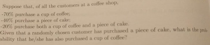
b.
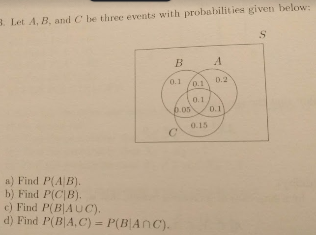
c.
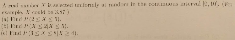
Problem 66-3
Estimated time: 30 min
Location: Overleaf
Grading: 10 points
Complete queries 1-5 in SQL Zoo Module 2. Take a screenshot of each successful query (with the successful smiley face showing) and put them in the overleaf doc.
Complete Module 8 of Sololearn's C++ Course. Take a screenshot of the completed module, with your user profile showing, and put it in the overleaf doc.
Problem 65-1
Estimated Time: 30 min
Location: Overleaf
Grading: 15 points
(Taken from Introduction to Probability: Statistics and Random Processes by Hossein Pishro-Nik)
a.
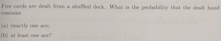
- Tip: for (b), compute $1-P(\textrm{complement}).$ Here, the complement is the event that you get no aces.
b.

- Tip: again, compute $1-P(\textrm{complement}).$
c.

Remember that PMF means "probability mass function". This is just the function $P(Z=z).$
Tip: Find the possible values of $Z,$ and then find the probabilities of those values of $Z$ occurring. Your answer will be a piecewise function: $$ P(z) = \begin{cases} \_\_\_, \, z=\_\_\_ \\ \_\_\_, \, z=\_\_\_ \\ \ldots \end{cases} $$
Problem 65-2
Estimated time: 30 min
Location: Overleaf
Grading: 5 points
Complete queries 11-15 in the SQL Zoo. Take a screenshot of each successful query (with the successful smiley face showing) and put them in the overleaf doc.
Complete Module 7 of Sololearn's C++ Course. Take a screenshot of the completed module, with your user profile showing, and put it in the overleaf doc.
Problem 64-1
Estimated time: 60 min
Location: assignment-problems/quicksort.py
Grading: 10 points
Previously, you wrote a variant of quicksort that involved splitting the list into two parts (one part $\leq$ the pivot, and another part $>$ the pivot), and then recursively calling quicksort on those parts.
However, this algorithm can be made more efficient by keeping everything in the same list (rather than creating two new lists). You can do this by swapping elements rather than breaking them out into new lists.
Your task is to write a quicksort algorithm that uses only one list, and uses swaps to re-order elements within that list, per the quicksort algorithm. Here is an example of how to do that.
Make sure your algorithm passes the same test as the quicksort without swaps (that you did on the previous assignment).
Problem 64-2
Estimated time: 30 min
Location: Overleaf
Grading: 10 points
Complete queries 1-10 in the SQL Zoo. Here's a reference for the LIKE operator, which will come in handy.
Take a screenshot of each successful query and put them in an overleaf doc. When a query is successful, you'll see a smiley face appear. Your screenshots should look like this:
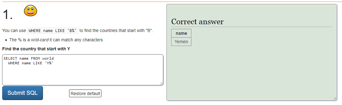
Problem 64-3
Estimated Time: 60 min
Location: Overleaf
Grading: 10 points
(Taken from Introduction to Probability: Statistics and Random Processes by Hossein Pishro-Nik)
a.
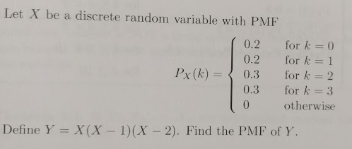
- The PMF tells you the probabilities of values of $X.$ For example, from the PMF, we have $P(X=0) = 0.2.$ You just need to plug in these values of $X$ into the function $Y=X(X-1)(X-2)$ and sum up any probabilities for which the same value of $Y$ is obtained.
b.
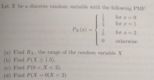
- Remember Bayes' rule: $P(A \, | \, B) = \dfrac{P(A \cap B)}{P(B)}$
c.
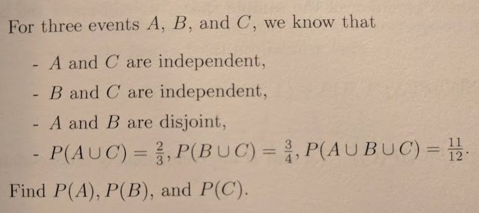
If two events $X$ and $Y$ are "independent", then $P(X \cap Y) = P(X) P(Y).$
If two events $X$ and $Y$ are "disjoint", then $P(X \cap Y) = 0.$
d.
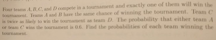
- Try setting up a system of equations.
Problem 64-4
Estimated Time: 15 min
Location: Overleaf
Grading: 5 points
(Taken from Introduction to Statistical Learning)
This problem is VERY similar to the test/train analysis you did in the previous assignment. But this time, you don't have to actually code up anything. You just have to use the concepts of overfitting and underfitting to justify your answers.
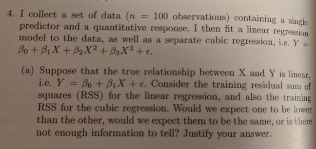
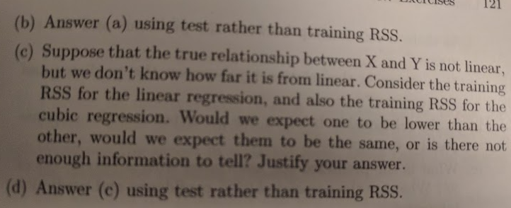
Problem 63-1
Grading: 20 points
(Taken from Introduction to Probability: Statistics and Random Processes by Hossein Pishro-Nik)
a.
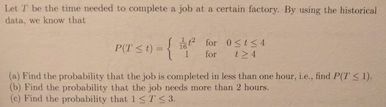
b.
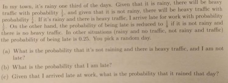
- This problem involves summing up probabilities over all possible paths that lead to a desired outcome. An easy way to do this is to use a tree diagram.
c.
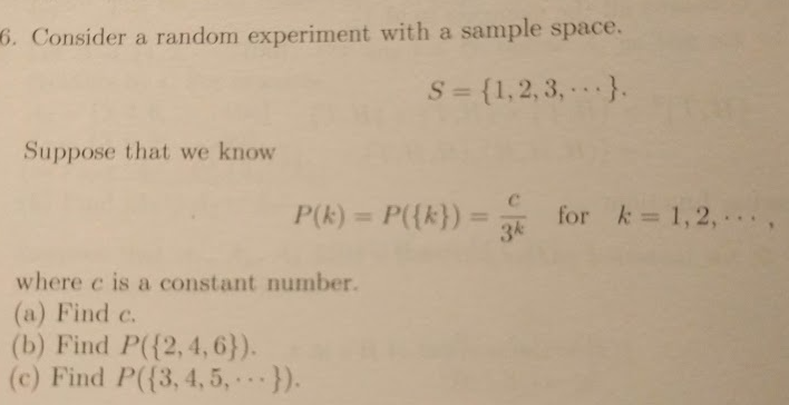
d.
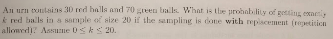
- Note: "with replacement" means that each time a ball is drawn, it is put back in for the next draw. So, it would be possible to draw the same ball more than once.
e.
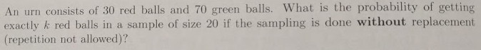
- Note: "without replacement" means that each time a ball is drawn, it is NOT put back in for the next draw. So, it would NOT be possible to draw the same ball more than once.
f.
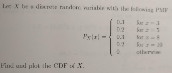
- Note: CDF stands for "Cumulative Distribution Function" and is defined as $\textrm{CDF}(x) = P(X \leq x).$
g.

Problem 63-2
Grading: 5 points
Complete Module 6 of Sololearn's C++ Course. Take a screenshot of the completed module, with your user profile showing, and submit it along with the assignment.
Complete Module 4 of Sololearn's SQL Course. Take a screenshot of the completed module, with your user profile showing, and submit it along with the assignment.
Problem 63-3
Grading: 5 points
Resolve the suggestions/comments on your blog post. Copy and paste everything back into Overleaf, and take a final proofread. Read it through to make sure everything is grammatically correct and makes sense. Submit your shareable Overleaf link along with the assignment.
Problem 62-1
Grading: 10 points
Create a class NaiveBayesClassifier withing machine-learning/src/naive_bayes_classifier.py that passes the following tests. These tests should be written in tests/test_naive_bayes_classifier.py using assert statements.
>>> df = DataFrame.from_array(
    [
        [False, False, False],
        [True, True, True],
        [True, True, True],
        [False, False, False],
        [False, True, False],
        [True, True, True],
        [True, False, False],
        [False, True, False],
        [True, False, True],
        [False, True, False]
    ]
    columns = ['errors', 'links', 'scam']
)
>>> naive_bayes = NaiveBayesClassifier(df, dependent_variable='scam')

>>> naive_bayes.probability('scam', True)
0.4
>>> naive_bayes.probability('scam', False)
0.6

>>> naive_bayes.conditional_probability(('errors',True), given=('scam',True))
1.0
>>> naive_bayes.conditional_probability(('links',False), given=('scam',True))
0.25

>>> naive_bayes.conditional_probability(('errors',True), given=('scam',False))
0.16666666666666666
>>> naive_bayes.conditional_probability(('links',False), given=('scam',False))
0.5

>>> observed_features = {
    'errors': True,
    'links': False
}
>>> naive_bayes.likelihood(('scam',True), observed_features)
0.1
>>> naive_bayes.likelihood(('scam',False), observed_features)
0.05

>>> naive_bayes.classify('scam', observed_features)
True

Note: in the event of a tie, choose the dependent variable that occurred most frequently in the dataset.
Problem 62-2
Grading: 10 points
Location: assignment-problems/quicksort_without_swaps.py
Implement a function quicksort that implements the variant of quicksort described here: https://www.youtube.com/watch?v=XE4VP_8Y0BU
- Note: this variant of
quicksortis very similar tomergesort.
Use your function to sort the list [5,8,-1,9,10,3.14,2,0,7,6] (write a test with an assert statement). Choose the pivot as the rightmost entry.
Problem 62-3
Grading: 10 points
Location: Writeup in Overleaf; code in machine-learning/analysis/assignment_62.py
Watch this video FIRST: https://youtu.be/EuBBz3bI-aA?t=29
a. Create a dataset as follows:
$$ \left\{ (x, y) \, \Bigg| \, \begin{matrix} x=0.1, 0.2, \ldots, 10 \\ y=3+0.5x^2 + \epsilon, \, \epsilon \sim \mathcal{U}(-5, 5) \end{matrix} \right\} $$Split the dataset into two subsets:
- a training dataset consisting of 80% of the data points, and
- a testing dataset consisting of 20% of the data points.
To do this, you can randomly remove 20% of the data points from the dataset.
b. Fit 5 models to the data: a linear regressor, a quadratic regressor, a cubic regressor, a quartic regressor, and a quintic regressor. Compute the residual sum of squares (RSS) for each model on the training data. Which model is most accurate on the training data? Explain why.
c. Compute the RSS for each model on the testing data. Which model is most accurate on the testing data? Explain why.
d. Based on your findings, which model is the best model for the data? Justify your choice.
Problem 61-1
Location: Overleaf
Grading: 10 points
Construct a decision tree model for the following data. Include the Gini impurity and goodness of split at each node. You should choose the splits so as to maximize the goodness of split each time. Also, draw a picture of the decision boundary on the graph.
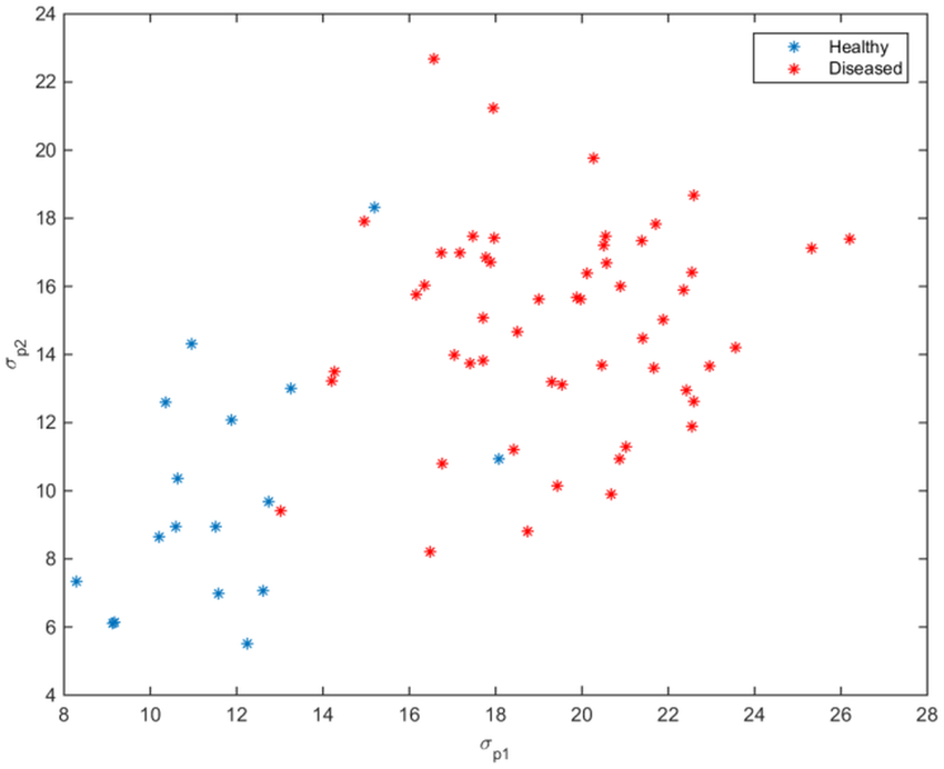
Problem 61-2
Location: simulation/analysis/3-neuron-network.py
Grading: 5 points
There are a couple things we need to update in our BiologicalNeuron and BiologicalNeuralNetwork, to make the model more realistic.
The first thing is that the synapse only releases neurotransmitters when a neuron has "fired". So, the voltage due to synapse inputs should not be a sum of all the raw voltages of the corresponding neurons. Instead, we should only sum the voltages that are over some threshold, say, $50 \, \textrm{mV}.$
So, our model becomes
$$\dfrac{\textrm dV}{\textrm dt} = \underbrace{\dfrac{1}{C} \left[ s(t) - I_{\text{Na}}(t) - I_{\text K}(t) - I_{\text L}(t) \right]}_\text{neuron in isolation} + \underbrace{\dfrac{1}{C} \left( \sum\limits_{\begin{matrix} \textrm{synapses from} \\ \textrm{other neurons} \\ \textrm{with } V(t) > 50 \end{matrix}} V_{\text{other neuron}}(t) \right)}_\text{interactions with other neurons}.$$Update your BiologicalNeuralNetwork using the above model. The resulting graph should stay mostly the same (but this update to the model will be important when we're simulating many neurons).
Problem 61-3
Grading: 5 points
Make suggestions on your assigned classmate's blog post. If anything is unclear, uninteresting, or awkwardly phrased, make a suggestion to improve it. You should the "suggesting" feature of Google Docs and type in how you would rephrase or rewrite the particular portions.
Be sure to look for and correct any grammar mistakes as well. This is the second round of review, so I'm expecting there to be NO grammar mistakes whatsoever after you're done reviewing.
Problem 61-4
Location: Overleaf
Grading: 5 points
(Taken from Introduction to Probability: Statistics and Random Processes by Hossein Pishro-Nik)
a.
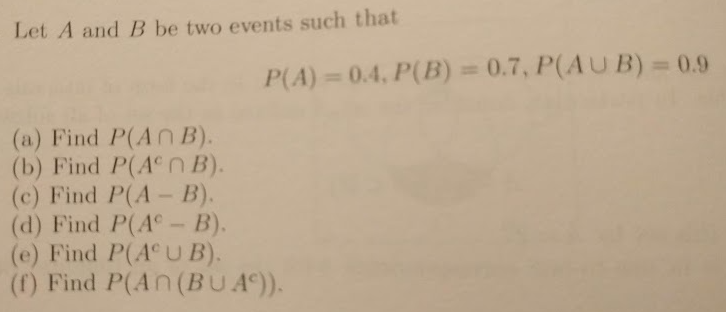
b.
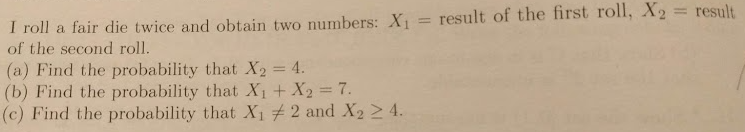
Problem 61-5
Grading: 5 points
Complete Module 3 of Sololearn's SQL Course. Take a screenshot of the completed module, with your user profile showing, and submit it along with the assignment.
Problem 60-1
Location: Overleaf
Grading: 5 points
For two positive functions $f(n)$ and $g(n),$ we say that $f = O(g)$ if
$$ \lim\limits_{n \to \infty} \dfrac{f(n)}{g(n)} < \infty, $$or equivalently, there exists a constant $c$ such that
$$ f(n) < c \cdot g(n) $$for all $n.$
Using the definition above, prove the following:
a. $3n^2 + 2n + 1 = O(n^2).$
b. If $O(f + g) = O(\max(f,g)).$
- Note: in your proof, you should show that if $h = O(f+g),$ then $h = O(\max(f,g)).$
c. $O(f) \cdot O(g) = O(f \cdot g).$
- Note: in your proof, you should show that if $x = O(f)$ and $y=O(g)$ and $h = O(f \cdot g),$ then $x \cdot y = O(h)$
d. If $f = O(g)$ and $g = O(h)$ then $f = O(h).$
Problem 60-2
Location: Overleaf
Grading: 5 points
(Taken from Introduction to Probability: Statistics and Random Processes by Hossein Pishro-Nik)
a.
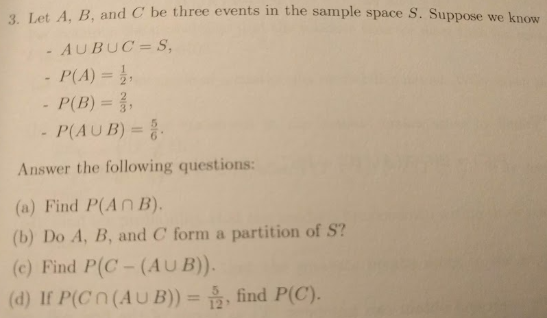
b.
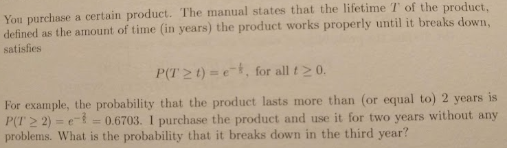
- Check: you should get a result of $0.1813.$ If you get stuck, then here's a link to a similar example, worked out.
c.
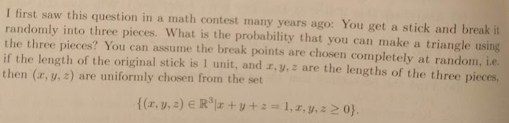
- Check: you should get a result of $1/4.$ Remember the triangle inequality! And remember that you can visualize this problem geometrically:
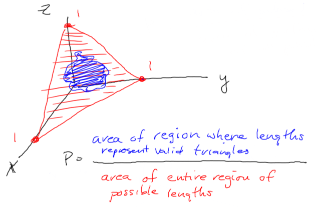
Problem 60-3
Location: Overleaf
Grading: 5 points
(Taken from Introduction to Statistical Learning)
IMPORTANT:
For part (a), write out the model for salary of a male in this dataset, and the model for salary of a female in this dataset, and use these models to justify your answer.
Perhaps counterintuitively, question (c) is false. I want you to provide a thorough explanation of why this is by coming up with a situation in which there would be a significant interaction, but the interaction term is small.
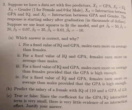
Problem 60-4
Grading: 5 points
Complete Module 5 of Sololearn's C++ Course. Take a screenshot of the completed module, with your user profile showing, and submit it along with the assignment.
Complete Module 2 of Sololearn's SQL Course. Take a screenshot of the completed module, with your user profile showing, and submit it along with the assignment.
Problem 60-5
Grading: 5 points (if you've completed these things already, then you get 5 points free)
Resolve any comments/suggestions in your blog post Google Doc
Catch up on any problems you haven't fully completed:
BiologicalNeuralNetwork,DumbPlayertests,percent_correctwithKNearestNeighborsClassifier
Problem 59-1
Location: Overleaf
Grading: 10 points
Construct a decision tree model for the following data, using the splits shown.
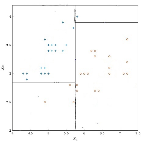
Remember that the formula for Gini impurity for a group with class distribution $\vec p$ is
$$ G(\vec p) = \sum_i p_i (1-p_i) $$and that the "goodness-of-split" is quantified as
$$ \text{goodness} = G(\vec p_\text{pre-split}) - \sum_\text{post-split groups} \dfrac{N_\text{group}}{N_\text{pre-split}} G(\vec p_\text{group}). $$See the updated Eurisko Assignment Template for an example of constructing a decision tree in latex for a graph with given splits.
Be sure to include the class counts, impurity, and goodness of split at each node
Be sure to label each edge with the corresponding decision criterion.
Problem 59-2
Grading: 10 points (5 points for writing tests, 5 points for passing tests)
Revise tests/test_dumb_player.py, so that it uses the actual game state. You can refer to Problem 23-3 for the tests.
For example, the first test is as follows:
At the end of Turn 1 Movement Phase:
    Player 0 has 3 scouts at (4,0)
    Player 1 has 3 scouts at (4,4)
Phrased in terms of the game state, we could write the test as
game_state = game.generate_state()
player_0_scout_locations = [u.location for u in game_state.players[0].units if unit.type == Scout]
player_1_scout_locations = [u.location for u in game_state.players[1].units if unit.type == Scout]
assert set(player_0_scout_locations) == set([(4,0), (4,0), (4,0)])
assert set(player_1_scout_locations) == set([(4,4), (4,4), (4,4)])
Given the refactoring that we've been doing, your tests might not run successfully the first time. But don't spend all your time on this problem only. If your tests don't pass, then make sure to complete all the other problems in this assignment before you start debugging your game.
Problem 59-3
Grading: 10 points
Make suggestions on your assigned classmate's blog post. If anything is unclear, uninteresting, or awkwardly phrased, make a suggestion to improve it. You should the "suggesting" feature of Google Docs and type in how you would rephrase or rewrite the particular portions.
Be sure to look for and correct any grammar mistakes as well. You'll be graded on how thorough your suggestions are. Everyone should be making plenty of suggestions (there's definitely at least 10 suggestions to be made on everyone's drafts).
Problem 59-4
Grading: 5 points
Complete Module 4 of Sololearn's C++ Course. Take a screenshot of the completed module, with your user profile showing, and submit it along with the assignment.
Complete Module 1 of Sololearn's SQL Course. Take a screenshot of the completed module, with your user profile showing, and submit it along with the assignment.
Problem 58-1
Grading: 10 points
Recall the following cookie dataset (that has been augmented with some additional examples):
['Cookie Type' ,'Portion Eggs','Portion Butter','Portion Sugar','Portion Flour' ]
[['Shortbread'  ,     0.14     ,       0.14     ,      0.28     ,     0.44      ],
['Shortbread'  ,     0.10     ,       0.18     ,      0.28     ,     0.44      ],
['Shortbread'  ,     0.12     ,       0.10     ,      0.33     ,     0.45      ],
['Shortbread'  ,     0.10     ,       0.25     ,      0.25     ,     0.40      ],
['Sugar'       ,     0.00     ,       0.10     ,      0.40     ,     0.50      ],
['Sugar'       ,     0.00     ,       0.20     ,      0.40     ,     0.40      ],
['Sugar'       ,     0.02     ,       0.08     ,      0.45     ,     0.45      ],
['Sugar'       ,     0.10     ,       0.15     ,      0.35     ,     0.40      ],
['Sugar'       ,     0.10     ,       0.08     ,      0.35     ,     0.47      ],
['Sugar'       ,     0.00     ,       0.05     ,      0.30     ,     0.65      ],
['Fortune'     ,     0.20     ,       0.00     ,      0.40     ,     0.40      ],
['Fortune'     ,     0.25     ,       0.10     ,      0.30     ,     0.35      ],
['Fortune'     ,     0.22     ,       0.15     ,      0.50     ,     0.13      ],
['Fortune'     ,     0.15     ,       0.20     ,      0.35     ,     0.30      ],
['Fortune'     ,     0.22     ,       0.00     ,      0.40     ,     0.38      ],
['Shortbread'  ,     0.05     ,       0.12     ,      0.28     ,     0.55      ],
['Shortbread'  ,     0.14     ,       0.27     ,      0.31     ,     0.28      ],
['Shortbread'  ,     0.15     ,       0.23     ,      0.30     ,     0.32      ],
['Shortbread'  ,     0.20     ,       0.10     ,      0.30     ,     0.40      ]]
When fitting our k-nearest neighbors models, we have been using this dataset to predict the type of a cookie based on its ingredient portions. We've also seen that issues can arise when $k$ is too small or too large.
So, what is a good value of $k?$
a. To explore this question, plot the function $$ y= \text{percent_correct}(k), \qquad k=1,2,3, \ldots, 16, $$ where $\text{percent_correct}(k)$ is the percentage of points in the dataset that the $k$-nearest neighbors model would classify correctly.
for each data point:
    1. fit a kNN model to all the data EXCEPT that data point
    2. use the kNN model to classify the data point
    3. determine whether the kNN classification matches up
       with the actual class of the data point

percent_correct = num_correct_classifications / tot_num_data_points
You should get the following result:
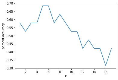
b. Based on what you know about what happens when $k$ is too small or too large, does the shape of your plot makes sense?
c. What would be an appropriate value (or range of values) of $k$ for this modeling task? Justify your answer by referring to your plot.
Problem 58-2
Grading: 10 points
Get your BiologicalNeuralNetwork fully working. Note that there's a particular issue with defining functions within for loops that Elijah pointed out on Slack:
Consider the following code:
funcs = []
for i in range(10):
    funcs.append(lambda x: x * i)
for f in funcs:
    print(f(5))
You'd expect to see 5, 10, 15, 20, 25, etc.
BUT what you actually get is 50, 50, 50, 50, 50, etc.
Instead ofi * 5, it is just doing10 * 5
This is because the lambda refers to the place thatiis stored in memory, which ends as10So instead of taking the current value ofiand using it in the lambda, it will take the last value it was set to, before it is actually called. The way you fix this problem is:funcs = [] for i in range(10): funcs.append(lambda x, i=i: x * i) for f in funcs: print(f(5))
So, when you're getting your derivatives, you'll need to do the following:
network_derivatives = []
for each neuron:

    parent_indices = indices of neurons that send synapses to neuron i

    # x is [V0, n0, m0, h0,
    #       V1, n1, m1, h1,
    #       V2, n2, m2, h2, ...]

    network_derivatives += [
        (
            lambda t, x, i=i, neuron=neuron:
                neuron.dV(t, x[4*i : (i+1)*4])
                + 1/neuron.C * sum(x[p*4] for p in parent_indices)
        ),
        (
            lambda t, x, i=i, neuron=neuron:
                neuron.dn(t, x[4*i : (i+1)*4])
        ),
        (
            lambda t, x, i=i, neuron=neuron:
                neuron.dm(t, x[4*i : (i+1)*4])
        ),
        (
            lambda t, x, i=i, neuron=neuron:
                neuron.dh(t, x[4*i : (i+1)*4])
        )
    ]
Problem 58-3
Grading: 10 points
For blog post draft #4, I want you to do the following:
George: Linear and Logistic Regression, Part 1: Understanding the Models
Make plots of the images you wanted to include, and insert them into your post. You can use character arguments in
plt.plot(); here's a referenceYou haven't really hit on why the logistic model takes a sigmoid shape. You should talk about the $e^{\beta x}$ term, where $\beta$ is negative. What happens when $x$ gets really negative? What happens when $x$ gets really positive?
For your linear regression, you should use coefficients $\beta_0, \beta_1, \ldots$ just like you did in the logistic regression. This will help drive the point home that logistic regression is just a transformation of linear regression.
We're ready to move onto the text editing phase! The next time you submit your blost, put it in a Google Doc and share it with me so that I can make "suggestions" on it.
Colby: Linear and Logistic Regression, Part 2: Fitting the Models
In your explanation of the pseudoinverse, make sure to state that in most modeling contexts, our matrix $X$ is taller than it is wide, because we have lots of data points. So our matrix $X$ is usually not invertible because it is a tall rectangular matrix.
In your explanation of the pseudoinverse, be more careful with your language: the pseudoinverse $(\mathbf{X}^T\mathbf{X})^{-1}$ is not equivalent to the standard inverse $\mathbf{X}^{-1}.$ The equation $\mathbf{X} \vec \beta = \vec y$ is usually not solvable, because the standard inverse $\mathbf{X}^{-1}$ usually does not exist. But the pseudoinverse $(\mathbf{X}^T\mathbf{X})^{-1}$ usually does exist, and the solution $\vec \beta = (\mathbf{X}^T\mathbf{X})^{-1} \mathbf{X}^T \vec y$ minimizes the sum of squared error between the desired output $\vec y$ and the actual output $\mathbf{X} \vec \beta.$
Decide between bracket matrices (
bmatrix) and parenthesis matrices (pmatrix). You sometiemes usebmatrix, and other timespmatrix. Choose one convention and stick to it.On page 2, show the following intermediate steps (fill in the dots): $$\begin{align*} \vec \beta &= \ldots \\ \vec \beta &= \begin{pmatrix} \cdot & \cdot & \cdot \\ \cdot & \cdot & \cdot \\ \cdot & \cdot & \cdot \end{pmatrix}^{-1} \begin{pmatrix} 1 & 1 & 1 & 1 \\ 0 & 1 & 0 & 4 \\ 0 & 0 & 2 & 5 \end{pmatrix} \begin{pmatrix} 0.1 \\ 0.2 \\ 0.5 \\ 0.6 \end{pmatrix} \\ \vec \beta &= \begin{pmatrix} \cdot & \cdot & \cdot & \cdot \\ \cdot & \cdot & \cdot & \cdot \\ \cdot & \cdot & \cdot & \cdot \\ \cdot & \cdot & \cdot & \cdot \end{pmatrix} \begin{pmatrix} 0.1 \\ 0.2 \\ 0.5 \\ 0.6 \end{pmatrix} \\ \vec \beta &= \ldots \end{align*}$$
Remove any parts of your code that are not relevant to the blog post (even if you used them for some part of an assignment). For example, you should remove the rounding part from
apply_coeffs.Make sure your code follows the same conventions everywhere. For example, you sometimes say
coefficients, and other times justcoeffs. For the purposes of this blog post, we want to be as clear as possible, so always usecoefficientsinstead ofcoeffs.Make your code tight so that there is zero redundancy. For example, in
__init__, the argumentratingsis redundant because these values are already in your dataframe, and you already have a variableprediction_columnthat indicates the relevant column in your dataframe. So eliminateratingsfrom your code.After you do the steps above, we're ready to move onto the text editing phase! The next time you submit your blog post, put it in a Google Doc and share it with me so that I can make "suggestions" on it.
Riley: Linear and Logistic Regression, Part 3: Categorical Variables, Interaction Terms, and Nonlinear Transformations of Variables
In the statements of your models, you need a constant term, and you need to standardize your coefficient labels and your variable names. You use different conventions in a lot of places -- sometimes you call the coefficients $a,b,c,\ldots,$ other times $c_1, c_2, c_3,\ldots,$ and other times $\beta_1,\beta_2,\beta_3,\ldots.$ Likewise, you sometimes say "beef" and "pb", while other times you say "roast beef" and "peanut butter". You need to standardize these names. I think using $\beta$'s or $c$'s for coefficients and abbreviations for variable names is preferable. So, for example, one of your equations would turn into $y = \beta_0 + \beta_1(\textrm{beef}) + \beta_2(\textrm{pb}) + \beta_3(\textrm{mayo}) + \beta_4(\textrm{jelly})$ or $y = c_0 + c_1(\textrm{beef}) + c_2(\textrm{pb}) + c_3(\textrm{mayo}) + c_4(\textrm{jelly}).$
After you do the steps above, we're ready to move onto the text editing phase! The next time you submit your blog post, put it in a Google Doc and share it with me so that I can make "suggestions" on it.
David: Predator-Prey Modeling with Euler Estimation
Explain this more clearly:
Euler estimation works by adding the derivative of an equation to each given value over and over again. This is because the derivatives are the instantaneous rates of change so we add it at each point to accurately show the the equation. Adding each point up from an equation is also equivalent to an integral.
Clean up your code on page 3. It's hard to tell what's going on. Put these code snippets into a single clean function, and change up the naming/structure so that it's clear what's going on. The code doesn't have to be the same as what's actually in your Euler estimator.
After you do the steps above, we're ready to move onto the text editing phase! The next time you submit your blog post, put it in a Google Doc and share it with me so that I can make "suggestions" on it.
Elijah: Solving Magic Squares using Backtracking
In your nested for loops, you should be using
range(1,10)because0is not considered as an element of the magic square.In your code snippets, you should name everything very descriptively so that it's totally obvious what things represent. For example, instead of
s = int(len(arr)**0.5), you could sayside_length = int(len(arr)**0.5).After you do the steps above, we're ready to move onto the text editing phase! The next time you submit your blog post, put it in a Google Doc and share it with me so that I can make "suggestions" on it.
Problem 57-1
Location: machine-learning/src/k_nearest_neighbors_classifier.py
Grading: 10 points
Create a class KNearestNeighborsClassifier that works as follows. Leverage existing methods in your DataFrame class to do the brunt of the processing.
>>> df = DataFrame.from_array(
    [['Shortbread'  ,     0.14     ,       0.14     ,      0.28     ,     0.44      ],
    ['Shortbread'  ,     0.10     ,       0.18     ,      0.28     ,     0.44      ],
    ['Shortbread'  ,     0.12     ,       0.10     ,      0.33     ,     0.45      ],
    ['Shortbread'  ,     0.10     ,       0.25     ,      0.25     ,     0.40      ],
    ['Sugar'       ,     0.00     ,       0.10     ,      0.40     ,     0.50      ],
    ['Sugar'       ,     0.00     ,       0.20     ,      0.40     ,     0.40      ],
    ['Sugar'       ,     0.10     ,       0.08     ,      0.35     ,     0.47      ],
    ['Sugar'       ,     0.00     ,       0.05     ,      0.30     ,     0.65      ],
    ['Fortune'     ,     0.20     ,       0.00     ,      0.40     ,     0.40      ],
    ['Fortune'     ,     0.25     ,       0.10     ,      0.30     ,     0.35      ],
    ['Fortune'     ,     0.22     ,       0.15     ,      0.50     ,     0.13      ],
    ['Fortune'     ,     0.15     ,       0.20     ,      0.35     ,     0.30      ],
    ['Fortune'     ,     0.22     ,       0.00     ,      0.40     ,     0.38      ]],
    columns = ['Cookie Type' ,'Portion Eggs','Portion Butter','Portion Sugar','Portion Flour' ]
    )
>>> knn = KNearestNeighborsClassifier(df, prediction_column = 'Cookie Type')
>>> observation = {
    'Portion Eggs': 0.10,
    'Portion Butter': 0.15,
    'Portion Sugar': 0.30,
    'Portion Flour': 0.45
}

>>> knn.compute_distances(observation)
Returns a dataframe representation of the following array:

[[0.047, 'Shortbread'],
 [0.037, 'Shortbread'],
 [0.062, 'Shortbread'],
 [0.122, 'Shortbread'],
 [0.158, 'Sugar'],
 [0.158, 'Sugar'],
 [0.088, 'Sugar'],
 [0.245, 'Sugar'],
 [0.212, 'Fortune'],
 [0.187, 'Fortune'],
 [0.396, 'Fortune'],
 [0.173, 'Fortune'],
 [0.228, 'Fortune']]

Note: the above has been rounded to 3 decimal places for ease of viewing, but you should not round yourself.

>>> knn.nearest_neighbors(observation)
Returns a dataframe representation of the following array:

[[0.037, 'Shortbread'],
 [0.047, 'Shortbread'],
 [0.062, 'Shortbread'],
 [0.088, 'Sugar'],
 [0.122, 'Shortbread'],
 [0.158, 'Sugar'],
 [0.158, 'Sugar'],
 [0.173, 'Fortune'],
 [0.187, 'Fortune'],
 [0.212, 'Fortune'],
 [0.228, 'Fortune'],
 [0.245, 'Sugar'],
 [0.396, 'Fortune']]

Note: the above has been rounded to 3 decimal places for ease of viewing, but you should not round yourself.

>>> knn.compute_average_distances(observation)

{
    'Shortbread': 0.067,
    'Sugar': 0.162,
    'Fortune': 0.239
}

Note: the above has been rounded to 3 decimal places for ease of viewing, but you should not round yourself.

>>> knn.classify(observation, k=5)
'Shortbread'

(In the case of a tie, chose whichever class has a lower average distance. If that is still a tie, then pick randomly.)
Problem 57-2
Location: simulation/analysis/3-neuron-network.py
Grading: 15 points
IMPORTANT UPDATE: I'm not going to take points off if your BiologicalNeuralNetwork isn't fully working. I'll expect to see at least the skeleton of it written, but there's this subtle thing with lambda functions that Elijah pointed out, that we need to talk about in class tomorrow.
Create a Github repository named simulation, and organize the code as follows:
simulation/
|- src/
   |- euler_estimatory.py
   |- biological_neuron.py
   |- biological_neural_network.py
|- tests/
   |- test_euler_estimator.py
|- analysis/
   |- predator_prey.py
   |- sir_epidemiology.py
Rename your class Neuron to be BiologicalNeuron. (This is to avoid confusion when we create another neuron class in the context of machine learning.)
Create a class BiologicalNeuralNetwork to simulate a network of interconnected neurons. This class will be initialized with two arguments:
neurons- a list of neurons in the networksynapses- a list of "directed edges" that correspond to connections between neurons
To simulate your BiologicalNeuralNetwork, you will use an EulerEstimator where x is a long array of V,n,m,h for each neuron. So, if you are simulating 3 neurons (neurons 0,1,2), then you will be passing in $4 \times 3 = 12$ derivatives:
Note that you will have to add extra terms to the voltage derivatives represent the synapses. The updated derivative of voltage is as follows: $$\dfrac{\textrm dV}{\textrm dt} = \underbrace{\dfrac{1}{C} \left[ s(t) - I_{\text{Na}}(t) - I_{\text K}(t) - I_{\text L}(t) \right]}_\text{neuron in isolation} + \underbrace{\dfrac{1}{C} \left( \sum\limits_{\begin{matrix} \textrm{synapses from} \\ \textrm{other neurons} \end{matrix}} V_{\text{other neuron}}(t) \right)}_\text{interactions with other neurons}.$$
So, in the case of 3 neurons connected as $0 \to 1 \to 2,$ the full system of equations would be as follows:
$$\begin{align*} \dfrac{\textrm dV_0}{\textrm dt} &= \textrm{neuron_0.dV}(V_0,n_0,m_0,h_0) \\ \dfrac{\textrm dn_0}{\textrm dt} &= \textrm{neuron_0.dn}(V_0,n_0,m_0,h_0) \\ \dfrac{\textrm dm_0}{\textrm dt} &= \textrm{neuron_0.dm}(V_0,n_0,m_0,h_0) \\ \dfrac{\textrm dh_0}{\textrm dt} &= \textrm{neuron_0.dh}(V_0,n_0,m_0,h_0) \\ \dfrac{\textrm dV_1}{\textrm dt} &= \textrm{neuron_1.dV}(V_1,n_1,m_1,h_1) + \dfrac{1}{\textrm{neuron_1.C}} V_0(t) \\ \dfrac{\textrm dn_1}{\textrm dt} &= \textrm{neuron_1.dn}(V_1,n_1,m_1,h_1) \\ \dfrac{\textrm dm_1}{\textrm dt} &= \textrm{neuron_1.dm}(V_1,n_1,m_1,h_1) \\ \dfrac{\textrm dh_1}{\textrm dt} &= \textrm{neuron_1.dh}(V_1,n_1,m_1,h_1) \\ \dfrac{\textrm dV_2}{\textrm dt} &= \textrm{neuron_2.dV}(V_2,n_2,m_2,h_2) + \dfrac{1}{\textrm{neuron_2.C}} V_1(t) \\ \dfrac{\textrm dn_2}{\textrm dt} &= \textrm{neuron_2.dn}(V_2,n_2,m_2,h_2) \\ \dfrac{\textrm dm_2}{\textrm dt} &= \textrm{neuron_2.dm}(V_2,n_2,m_2,h_2) \\ \dfrac{\textrm dh_2}{\textrm dt} &= \textrm{neuron_2.dh}(V_2,n_2,m_2,h_2) \end{align*}$$Test your BiologicalNeuralNetwork as follows:
>>> def electrode_voltage(t):
        if t > 10 and t < 11:
            return 150
        elif t > 20 and t < 21:
            return 150
        elif t > 30 and t < 40:
            return 150
        elif t > 50 and t < 51:
            return 150
        elif t > 53 and t < 54:
            return 150
        elif t > 56 and t < 57:
            return 150
        elif t > 59 and t < 60:
            return 150
        elif t > 62 and t < 63:
            return 150
        elif t > 65 and t < 66:
            return 150
        return 0

>>> neuron_0 = BiologicalNeuron(stimulus = electrode_voltage)
>>> neuron_1 = BiologicalNeuron()
>>> neuron_2 = BiologicalNeuron()
>>> neurons = [neuron_0, neuron_1, neuron_2]

>>> synapses = [(0,1), (1,2)]
The neural network resembles a directed graph:
0 --> 1 --> 2

>>> network = BiologicalNeuralNetwork(neurons, synapses)
>>> euler = EulerEstimator(
        derivatives = network.get_derivatives(),
        point = network.get_starting_point()
    )
>>> plt.plot([n/2 for n in range(160)], [electrode_voltage(n/2) for n in range(160)])
>>> euler.plot([0, 80], step_size = 0.001)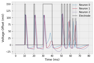
Problem 57-3
Grading: 5 points
Complete Module 3 of Sololearn's C++ Course. Take a screenshot of the completed module, with your user profile showing, and submit it along with the assignment.
Problem 56-1
Location: machine-learning/tests/test_data_frame.py
Grading: 10 points
Implement the following functionality in your DataFrame, and assert that these tests pass.
a. Loading an array. You'll need to use @classmethod for this one (read about it here).
>>> columns = ['firstname', 'lastname', 'age']
>>> arr = [['Kevin', 'Fray', 5],
           ['Charles', 'Trapp', 17],
           ['Anna', 'Smith', 13],
           ['Sylvia', 'Mendez', 9]]
>>> df = DataFrame.from_array(arr, columns)
b. Selecting columns by name
>>> df.select_columns(['firstname','age']).to_array()
[['Kevin', 5],
['Charles', 17],
['Anna', 13],
['Sylvia', 9]]
c. Selecting rows by index
>>> df.select_rows([1,3]).to_array()
[['Charles', 'Trapp', 17],
['Sylvia', 'Mendez', 9]]
d. Selecting rows which satisfy a particular condition (given as a lambda function)
>>> df.select_rows_where(
    lambda row: len(row['firstname']) >= len(row['lastname'])
                and row['age'] > 10
    ).to_array()
[['Charles', 'Trapp', 17]]
e. Ordering the rows by given column
>>> df.order_by('age', ascending=True).to_array()
[['Kevin', 'Fray', 5],
['Sylvia', 'Mendez', 9],
['Anna', 'Smith', 13],
['Charles', 'Trapp', 17]]

>>> df.order_by('firstname', ascending=False).to_array()
[['Sylvia', 'Mendez', 9],
['Kevin', 'Fray', 5],
['Charles', 'Trapp', 17],
['Anna', 'Smith', 13]]
Problem 56-2
Grading: 10 points
For blog post draft #3, I want you to do the following:
George: Linear and Logistic Regression, Part 1: Understanding the Models
Make plots of the images you wanted to include, and insert them into your post. You can use character arguments in
plt.plot(); here's a referenceYou haven't really hit on why the logistic model takes a sigmoid shape. You should talk about the $e^{\beta x}$ term, where $\beta$ is negative. What happens when $x$ gets really negative? What happens when $x$ gets really positive?
For your linear regression, you should use coefficients $\beta_0, \beta_1, \ldots$ just like you did in the logistic regression. This will help drive the point home that logistic regression is just a transformation of linear regression.
We're ready to move onto the text editing phase! The next time you submit your blost, put it in a Google Doc and share it with me so that I can make "suggestions" on it.
Colby: Linear and Logistic Regression, Part 2: Fitting the Models
You haven't defined what $y'$ means. Be sure to do that
You've got run-on sentences and incorrect comma usage everywhere. Fix that. Read each sentence aloud and make sure it makes sense as a complete sentence.
In your explanation of the pseudoinverse, you say that it's a generalization of the matrix inverse when the matrix may not be invertible. That's correct. But you should also explain why, in our case, the matrix $X$ is not expected to be invertible. (Think: only square matrices are invertible. Is $X$ square?)
Your matrix entries are backwards. For example, the first row should be $x_{11}, x_{12}, \ldots, x_{1n}.$
Wherever you use
ln, you should use\lninstead.In your linear/logistic regression functions, you should use $x_1, x_2, \ldots, x_m$ instead of $a,b, \ldots z.$
In your examples of the linear and logistic regression, you should use 3-dimensional data points instead of just 2-dimensional data point. This way, your example can demonstrate how you deal with multiple input variables. Also, you should set up some context around the example. Come up with a concrete situation in which your data points could be observations, and you want to predict something.
Riley: Linear and Logistic Regression, Part 3: Categorical Variables, Interaction Terms, and Nonlinear Transformations of Variables
Instead of inserting a screenshot of the raw data, put it in a data table. See the template for how to create data tables.
You have some models in text:
y = a(roast beef)+b(peanut butter)andy = a(roast beef)+b(peanut butter)+c(roast beef)(peanut butter).These should be on their own lines, as equations.There are some sections where the wording is really confusing. Proofread your paper and make sure that everything is expressed clearly. For example, this is not expressed clearly:
So for example we could not regress y = x^a. The most important attribute of this is that we can plot a logistic regression using this method. This is possible because the format of the logistic regression is ....At the very end, when you talk about transforming a dataset to fit a quadratic, it's not clear what you're doing. (I know what you're trying to say, but if I didn't already know, then I'd probably be confused.) You should explain how, in general, if we want to fit a nonlinear regression model $$ y= \beta_1 f_2(x_1) + \beta_2 f_2(x_2) + \cdots, $$ then we have to transform the data as $$ (x_1, x_2, \ldots ,y) \to (f_1(x_1), f_2(x_2), \ldots, y) $$ and then fit a linear regression to the points of the form $(f_1(x_1), f_2(x_2), \ldots, y).$
David: Predator-Prey Modeling with Euler Estimation
Fix your latex formatting -- follow the latex commandments.
Use pseudocode formatting (see the template)
In the predator-prey model that you stated, you need to explain where each term comes from. You've sort of hit on this below the model, but you haven't explicitly paired each individual term with its explanation. Also, why do we multiply the $DW$ together for some of the terms? Imagine that the reader knows what a derivative is, but has no experience using a differential equation for modeling purposes.
You should also explain that this equation is difficult to solve analytically, so that's why we're going to turn to Euler estimation.
You should explain where these recurrences come from. Why does this provide a good estimation of the function? (You should talk about rates of change) $$\begin{align*}D(t + \Delta t) &\approx D(t) + D'(t) \Delta t \\ W(t + \Delta t) &\approx W(t) + W'(t) \Delta t \end{align*}$$
When explaining Euler estimation, you should show the computations for the first few points in the plot. This way, the reader can see a concrete example of the process that you're actually carrying out to generate the plot.
Elijah: Solving Magic Squares using Backtracking
Make sure that the rest of your content is there on the next draft:
How can you overcome the inefficiency of brute-force search using "backtracking", i.e. intelligent search? https://en.wikipedia.org/wiki/Sudoku_solving_algorithms#Backtracking
Write some code for how to implement backtracking using a bunch of nested for loops (i.e. the ugly solution). Run some actual simulations to see how long it takes you to find a solution to a 3x3 magic square using backtracking. Then try the 4x4, 5x5, etc and make a graph.
How can you write the code more compactly using a single while loop?
Problem 56-3
Complete Module 1 AND Module 2 of Sololearn's C++ Course. Take a screenshot of each completed module, with your user profile showing, and submit both screenshots along with the assignment.


Problem 55-1
Location: Overleaf
Grading: 12 points
Naive Bayes classification is a way to classify a new observation consisting of multiple features, if we have data about how other observations were classified. It involves choosing the class that maximizes the posterior distribution of the classes, given the observation.
$$\begin{align*} \text{class} &= \underset{\text{class}}{\arg\max} \, P(\text{class} \, | \, \text{observed features}) \\ &= \underset{\text{class}}{\arg\max} \, \dfrac{P(\text{observed features} \, | \, \text{class}) P(\text{class})}{P(\text{observed features})} \\ &= \underset{\text{class}}{\arg\max} \, P(\text{observed features} \, | \, \text{class}) P(\text{class})\\ &= \underset{\text{class}}{\arg\max} \, \prod\limits_{\text{observed}\\ \text{features}} P(\text{feature} \, | \, \text{class}) P(\text{class})\\ &= \underset{\text{class}}{\arg\max} \, P(\text{class}) \prod\limits_{\text{observed}\\ \text{features}} P(\text{feature} \, | \, \text{class}) \\ \end{align*}$$The key assumption (used in the final line) is that all the features are independent:
$$\begin{align*} P(\text{observed features} \, | \, \text{class}) = \prod\limits_{\text{observed} \\ \text{features}} P(\text{feature} \, | \, \text{class}) \end{align*}$$Suppose that you want to find a way to classify whether an email is a phishing scam or not, based on whether it has errors and whether it contains links.
After checking 10 emails in your inbox, you came up with the following data set:
- No errors, no links; NOT scam
- Contains errors, contains links; SCAM
- Contains errors, contains links; SCAM
- No errors, no links; NOT scam
- No errors, contains links; NOT scam
- Contains errors, contains links; SCAM
- Contains errors, no links; NOT scam
- No errors, contains links; NOT scam
- Contains errors, no links; SCAM
- No errors, contains links; NOT scam
Now, you look at 4 new emails. For each of the new emails, compute
$$ P(\text{scam}) \prod\limits_{\text{observed}\\ \text{features}} P(\text{feature} \, | \, \text{scam}) \\[10pt] \text{and} \\[10pt] P(\text{not scam}) \prod\limits_{\text{observed}\\ \text{features}} P(\text{feature} \, | \, \text{not scam}) $$and decide whether it is a scam.
a. No errors, no links. You should get
$$ P(\text{scam}) \prod\limits_{\text{observed}\\ \text{features}} P(\text{feature} \, | \, \text{scam}) = 0 \\[10pt] \text{and} \\[10pt] P(\text{not scam}) \prod\limits_{\text{observed}\\ \text{features}} P(\text{feature} \, | \, \text{not scam}) = \dfrac{1}{4}. $$b. Contains errors, contains links. You should get
$$ P(\text{scam}) \prod\limits_{\text{observed}\\ \text{features}} P(\text{feature} \, | \, \text{scam}) = \dfrac{3}{10} \\[10pt] \text{and} \\[10pt] P(\text{not scam}) \prod\limits_{\text{observed}\\ \text{features}} P(\text{feature} \, | \, \text{not scam}) = \dfrac{1}{20}. $$c. Contains errors, no links. You should get
$$ P(\text{scam}) \prod\limits_{\text{observed}\\ \text{features}} P(\text{feature} \, | \, \text{scam}) = \dfrac{1}{10} \\[10pt] \text{and} \\[10pt] P(\text{not scam}) \prod\limits_{\text{observed}\\ \text{features}} P(\text{feature} \, | \, \text{not scam}) = \dfrac{1}{20}. $$d. No errors, contains links. You should get
$$ P(\text{scam}) \prod\limits_{\text{observed}\\ \text{features}} P(\text{feature} \, | \, \text{scam}) = 0 \\[10pt] \text{and} \\[10pt] P(\text{not scam}) \prod\limits_{\text{observed}\\ \text{features}} P(\text{feature} \, | \, \text{not scam}) = \dfrac{1}{4}. $$Problem 55-2
Grading: 12 points
Refactor your Hodgkin-Huxley neuron simulation so that the functions governing the internal state of the neuron are encapsulated within a class Neuron.
>>> def stimulus(t):
        if t > 10 and t < 11:
            return 150
        elif t > 20 and t < 21:
            return 150
        elif t > 30 and t < 40:
            return 150
        elif t > 50 and t < 51:
            return 150
        elif t > 53 and t < 54:
            return 150
        elif t > 56 and t < 57:
            return 150
        elif t > 59 and t < 60:
            return 150
        elif t > 62 and t < 63:
            return 150
        elif t > 65 and t < 66:
            return 150
        return 0
>>> neuron = Neuron(stimulus)
>>> neuron.plot_activity()
The above code should generate the SAME plot that you generated previously.
Note: Do NOT make plot_activity() into a gigantic function. Rather, you should keep your code modular, using helper functions when appropriate. Multiple helper functions will be needed to achieve this implementation with good code quality.
Problem 55-3
Grading: 6 points
Create an EconomicEngine that handles the following:
- CP income
- maintenance costs
- ship removals
- ship/technology purchases
This will be in the spirit of how MovementEngine handles movement and CombatEngine handles combat.
In your EconomicEngine, include a method generate_economic_state() that generates the following information:
economic_state = {
    'income': 20,
    'maintenance cost': 5
}
Problem 54-1
Location: Overleaf
Grading: 10 points
Note: Points will be deducted for poor latex quality. If you're writing up your latex and anything looks off, make sure to post about it so you can fix it before you submit. FOLLOW THE LATEX COMMANDMENTS!
The dataset below displays the ratio of ingredients for various cookie recipes.
['ID', 'Cookie Type' ,'Portion Eggs','Portion Butter','Portion Sugar','Portion Flour' ]

[[ 1 , 'Shortbread'  ,     0.14     ,       0.14     ,      0.28     ,     0.44      ],
[ 2  , 'Shortbread'  ,     0.10     ,       0.18     ,      0.28     ,     0.44      ],
[ 3  , 'Shortbread'  ,     0.12     ,       0.10     ,      0.33     ,     0.45      ],
[ 4  , 'Shortbread'  ,     0.10     ,       0.25     ,      0.25     ,     0.40      ],
[ 5  , 'Sugar'       ,     0.00     ,       0.10     ,      0.40     ,     0.50      ],
[ 6  , 'Sugar'       ,     0.00     ,       0.20     ,      0.40     ,     0.40      ],
[ 7  , 'Sugar'       ,     0.10     ,       0.08     ,      0.35     ,     0.47      ],
[ 8  , 'Sugar'       ,     0.00     ,       0.05     ,      0.30     ,     0.65      ],
[ 9  , 'Fortune'     ,     0.20     ,       0.00     ,      0.40     ,     0.40      ],
[ 10 , 'Fortune'     ,     0.25     ,       0.10     ,      0.30     ,     0.35      ],
[ 11 , 'Fortune'     ,     0.22     ,       0.15     ,      0.50     ,     0.13      ],
[ 12 , 'Fortune'     ,     0.15     ,       0.20     ,      0.35     ,     0.30      ],
[ 13 , 'Fortune'     ,     0.22     ,       0.00     ,      0.40     ,     0.38      ]]
Suppose you're given a cookie recipe and you want to determine whether it is a shortbread cookie, a sugar cookie, or a fortune cookie. The cookie recipe consists of 0.10 portion eggs, 0.15 portion butter, 0.30 portion sugar, and 0.45 portion flour. We will infer the classification of this cookie using the "$k$ nearest neighbors" approach.
Part 1: How to do $k$ nearest neighbors.
a. This cookie can be represented as the point $P(0.10, 0.15, 0.30, 0.45).$ Compute the Euclidean distance between $P$ and each of the points corresponding to cookies in the dataset.
- NOTE: YOU DON'T HAVE TO SHOW YOUR CALCULATIONS. Just write a Python script to do the calculations for you and print out the results, and in your writeup you can just include the final results.
b. Consider the 5 points that are closest to $P.$ (These are the 5 "nearest neighbors".) What cookie IDs are they, and what types of cookies are represented by these points?
c. What cookie classification showed up most often in the 5 nearest neighbors? What inference can you make about the recipe corresponding to the point $P$?
Part 2: The danger of using too large a $k$
a. What happens if we try to perform the $k$ nearest neighbors approach with $k=13$ (i.e. the full dataset) to infer the cookie classification of point $P?$ What issue occurs, and why does it occur?
b. For each classification of cookie, find the average distance between $P$ and the points corresponding to the cookies in that classification. Explain how this resolves the issue you identified in part (a).
Problem 54-2
Location: Overleaf
Grading: 10 points
Note: Points will be deducted for poor latex quality. If you're writing up your latex and anything looks off, make sure to post about it so you can fix it before you submit. FOLLOW THE LATEX COMMANDMENTS!
Suppose you want to estimate the probability that you will get into a particular competitive college. You had a bunch of friends a year ahead of you that applied to the college, and these are their results:
Martha was accepted. She was the 95th percentile of her class, got a 33 on the ACT, and had an internship at a well-known company the summer before she applied to college.
Jeremy was rejected. He was in the 95th percentile of his class and got a 34 on the ACT.
Alphie was accepted. He was in the 92nd percentile of his class, got a 35 on the ACT, and had agreed to play on the college's basketball team if accepted.
Dennis was rejected. He was in the 85th percentile of his class, got a 30 on the ACT, and had committed to run on the college's track team if accepted.
Jennifer was accepted. She was in the 80th percentile of her class, got a 36 on the ACT, and had a side business in 3D printing that was making $15,000 per year.
Martin was rejected. He was in the 85th percentile of his class, got a 29 on the ACT, and had was a finalist in an international science fair.
Mary was accepted. She was in the 95th percentile of her class, got a 36 on the ACT, and was a national finalist in the math olympiad.
Dean was rejected. He was in the 87th percentile of his class, got a 31 on the ACT, and was a national finalist in the chemistry olympiad.
Adam was accepted. He was in the 99th percentile of his class and got a 36 on the ACT.
Jeremy was rejected. He was in the 95th percentile of his class and got a 32 on the ACT.
Create a writeup in Overleaf that contains the following parts.
a. Create a quantitative dataset to represent this information, and include it in your writeup. Name your features appropriately.
Important: If you use 0 as the output for rejections and 1 as the output for acceptances, you do run into a problem where the regressor blows up. One solution is to use a small number like 0.001 for rejections and 0.999 for acceptances. But like Elijah pointed out, if you change that number to 0.0000001 or something else, then some of the outputs can drastically change.
But think about the college admissions process for these students: given these students' stats, how sure can you actually be that they will or won't get into a college? For example, 0.999999999 seems extreme because you can't be 99.9999999% sure you'll get into a competitive college. Something like, say, in the ballpark of 80% seems more reasonable as a max certainty. So instead of using 0's and 1's in your dataset, you should change those to numbers that would give a more realistic representation of the min certainty & max certainty that these students would get into the college.
There's not really a single correct answer, but you do need to provide some reasonable justification for the numbers that you chose to represent min and max acceptance probability. There's a saying that applies here: "All models are wrong, but some are useful".
b. Decide what type of model you will use to model the probability of acceptance as a function of the features in your dataset. State and justify the form of the model in your writeup.
c. Fit the model to the data. For each feature, answer the following questions:
According to your model, as that variable increases, does the estimated probability of acceptance increase or decrease? Does that result make sense? If so, why? (If not, then something is wrong with your model, and you need to figure out what's going wrong.)
d. Estimate the probability of being accepted for each of the data points that you used to fit the model. How well does this match up with reality?
e. Estimate your probability of being accepted if you are in the 95th percentile of your class and got a 34 on the ACT. Justify why your model's prediction is reasonable.
f. Now suppose that you have an opportunity to do an internship at a well-known company the summer before you apply to college. If you do it, what will your estimated probability of acceptance become? Based on this information, how much does the internship matter in terms of getting into the college you want?
Problem 54-3
Grading: 10 points
For blog post draft #2, I want you to finish addressing all of the key parts in the content. We'll worry about grammar / phrasing / writing style later.
Here are the things that you still need to address...
George: Linear and Logistic Regression, Part 1: Understanding the Models
You've talked about what regression can be used for. But what exactly is regression? In the beginning, you should write a bit about how regression involves fitting a function to the "general trend" of some data points, and then using that function to predict outcomes for data points where the outcome is not already known.
You should state the linear regression model before you state the logistic regression model, because linear regression is much simpler.
You've given the logistic regression model and stated its sigmoid shape. You should write a bit about why the model takes that shape. Explain why that form of function gives rise to a sigmoid shape.
You should also state how the two models can be generalized when there are multiple input variables.
You've stated that you can change the upper limit of the logistic regression, and you've given some examples of why you might want to do this, but you haven't actually explained how you do this in the equation. What number do you have to change?
Still need to do this: Explain how a logistic model can be adjusted to model variables that range from some general lower bound $a$ to some general upper bound $b.$ Give a couple examples of situations in which we'd want to do this.
Colby: Linear and Logistic Regression, Part 2: Fitting the Models
You've stated the matrix equation for linear regression, but you should explain a bit where it comes from. What is the system of equations you start with, and why does that correspond to the matrix equation you stated?
You've used the term "pseudoinverse" but you haven't stated exactly what that is in the equation. In particular: why do you have to multiply both sides by the transpose first? How come you couldn't just invert the matrix right off the bat?
You've stated that for the logistic regressor, the process is similar, but you have to transform y. But why do you transform y in this way? You need to start with the logistic regression equation, invert it, and then write down the system of equations. Then you can explain how this now looks like a linear regression, except that the right-hand side is just a transformation of y.
Riley: Linear and Logistic Regression, Part 3: Categorical Variables, Interaction Terms, and Nonlinear Transformations of Variables
Separate your text into paragraphs.
Typeset your math markup, putting equations on separate lines where appropriate.
David: Predator-Prey Modeling with Euler Estimation
In the predator-prey model that you stated, you need to explain where each term comes from. You've sort of hit on this below the model, but you haven't explicitly paired each individual term with its explanation. Also, why do we multiply the $DW$ together for some of the terms? Imagine that the reader knows what a derivative is, but has no experience using a differential equation for modeling purposes.
After you set up the system, you should start talking about the Euler estimation process. The plot should come at the very end, because it's the "punch line" of the blog post. You should also explain that this equation is difficult to solve analytically, so that's why we're going to turn to Euler estimation.
It looks like you've got some code snippets in an equation environment. Use the code environment provided in the template (I've updated the template recently). The code will look much better that way.
Before you dive into your code explanation of Euler estimation, you should do a brief mathematical explanation, referencing the main recurrences: $D(t + \Delta t) \approx D(t) + D'(t) \Delta t,$ $W(t + \Delta t) \approx W(t) + W'(t) \Delta t.$ You should also explain where these recurrences come from.
When explaining Euler estimation, you should show the computations for the first few points in the plot. This way, the reader can see a concrete example of the process that you're actually carrying out to generate the plot.
Elijah: Solving Magic Squares using Backtracking
Continue writing the rest of your draft. Here are the areas you still need to address:
How do you write the
is_validfunction?What's the problem with brute-force search? Run some actual simulations to see how long it takes you to find a solution to a 3x3 magic square using brute force. Then try the 4x4, 5x5, etc and make a graph. State the results as something ridiculous -- e.g. (it'll take me years to solve a something-by-something magic square)
What is the most obvious inefficiency in brute-force search? (It spends a lot of time exploring invalid combinations.)
How can you overcome this inefficiency using "backtracking", i.e. intelligent search? https://en.wikipedia.org/wiki/Sudoku_solving_algorithms#Backtracking
Write some code for how to implement backtracking using a bunch of nested for loops (i.e. the ugly solution). Run some actual simulations to see how long it takes you to find a solution to a 3x3 magic square using backtracking. Then try the 4x4, 5x5, etc and make a graph.
How can you write the code more compactly using a single while loop?
Problem 53-1
Location: Overleaf
Grading: 2 points for each part
Note: Points will be deducted for poor latex quality. If you're writing up your latex and anything looks off, make sure to post about it so you can fix it before you submit. FOLLOW THE LATEX COMMANDMENTS!
a. The covariance of two random variables $X_1,X_2$ is defined as
$$\text{Cov}[X_1,X_2] = \text{E}[(X_1 - \overline{X}_1)(X_2 - \overline{X}_2)].$$Given that $X \sim U[0,1],$ compute $\text{Cov}[X,X^2].$
- You should get a result of $\dfrac{1}{12}.$
b. Given that $X_1, X_2 \sim U[0,1],$ compute $\text{Cov}[X_1, X_2].$
- You should get a result of $0.$ (It will always turn out that the covariance of independent random variables is zero.)
c. Prove that
$$\text{Var}[X_1 + X_2] = \text{Var}[X_1] + \text{Var}[X_2] + 2 \text{Cov}[X_1,X_2].$$d. Prove that
$$\text{Cov}[X_1,X_2] = E[X_1 X_2] - E[X_1] E[X_2].$$Problem 53-2
Grading: 7 points
Create a MovementEngine that handles the movement of ships, similar to how CombatEngine handles combat.
In your MovementEngine, include a method generate_movement_state() that generates the following information:
movement_state = {
    'round': 1, # Movement 1, 2, or 3
}
For now, most of the relevant information (e.g. the locations of ships) will already be included in the game state. But we may want to expand the movement state in the future, as we include more features of the game.
Problem 53-3
Grading: 1 point
Email me a bio AND a headshot that you want to be included on the website: https://eurisko.us/people/
Here's a sample, if you want to use a similar structure:
John Doe is a sophomore in Math Academy and App Academy at Pasadena High School. Outside of school, he enjoys running the 100m and 200m sprints in track, playing video games, and working on his Eagle Scout project that involves saving the lives of puppies from students who don’t regularly commit their Github code. For college, John wants to study math and computer science.
Problem 52-1
Location: Overleaf
NOTE: Points will be deducted for poor latex quality.
a. (2 points) Using the identity $\text{Var}[X] = \text{E}[X^2] - \text{E}[X]^2,$ compute $\text{Var}[X]$ if $X$ is sampled from the continuous uniform distribution $U[a,b].$
- You should get the same result that you've gotten previously, using the definition of variance.
b. (2 points) Using the identity $\text{Var}[X] = \text{E}[X^2] - \text{E}[X]^2,$ compute $\text{Var}[X]$ if $X$ is sampled from the exponential distribution $p(x) = \lambda e^{-\lambda x}, \, x \geq 0.$
- You should get the same result that you've gotten previously, using the definition of variance.
c. (2 points) Using the identity $\text{Var}[N] = \text{E}[N^2] - \text{E}[N]^2,$ compute $\text{Var}[N]$ if $N$ is sampled from the Poisson distribution $p(n) = \dfrac{\lambda^n e^{-\lambda}}{n!}, \, n \in \left\{ 0, 1, 2, \ldots \right\}.$
- You should get the same result that you've gotten previously, using the definition of variance.
Problem 52-2
Location: assignment-problems/hodgkin_huxley.py
Grading: 14 points
The Nobel Prize in Physiology or Medicine 1963 was awarded jointly to Sir John Carew Eccles, Alan Lloyd Hodgkin and Andrew Fielding Huxley for their 1952 model of "spikes" (called "action potentials") in the voltage of neurons, using differential equations.
Watch this video to learn about neurons, and this video to learn about action potentials.
Here is a link to the Hodgkin-Huxley paper. I've outlined the key points of the model below.
Idea 0: Start with physics fundamentals
From physics, we know that current is proportional to voltage by a constant $C$ called the capacitance:
$$I(t) = C \dfrac{\textrm dV}{\textrm dt}$$So, the voltage of a neuron can be modeled as
$$\dfrac{\textrm dV}{\textrm dt} = \dfrac{I(t)}{C}.$$For neurons, we have $C \approx 1.0 \, .$
Idea 1: Decompose the current into 4 main subcurrents (stimulus & ion channels)
The current $I(t)$ consists of
a stimulus $s(t)$ to the neuron (from an electrode or other neurons),
current flux across sodium and potassium ion channels ($I_{\text{Na}}(t)$ and $I_{\text K}(t)$), and
current leakage, treated as a channel $I_{\text L}(t).$
So, we have
$$\dfrac{\textrm dV}{\textrm dt} = \dfrac{1}{C} \left[ s(t) - I_{\text{Na}}(t) - I_{\text K}(t) - I_{\text L}(t) \right].$$
Idea 2: Model the ion channel currents
The current across an ion channel is proportional to the voltange difference, relative to the equilibrium voltage of that channel:
$$\begin{align*} I_{\text{Na}}(t) &= g_{\text{Na}}(t) \left( V(t) - V_\text{Na} \right), \quad& I_{\text{K}}(t) &= g_{\text{K}}(t) \left( V(t) - V_\text{K} \right), \quad& I_{\text{L}}(t) &= g_{\text{L}}(t) \left( V(t) - V_\text{L} \right), \\ V_\text{Na} &\approx 115, \quad& V_\text{K} &\approx -12, \quad& V_\text{L} &\approx 10.6 \end{align*}$$The constants of proportionality are conductances, which were modeled experimentally:
$$\begin{align} g_{\text{Na}}(t) &= \overline{g}_{\text{Na}} m(t)^3 h(t), \quad& g_{\text{K}}(t) &= \overline{g}_{\text{K}} n(t)^4, \quad& g_{\text L}(t) &= \overline{g}_\text{L}, \\ \overline{g}_{\text{Na}} &\approx 120, \quad& \overline{g}_{\text{K}} &\approx 36, \quad& \overline{g}_{\text{L}} &\approx 0.3, \end{align}$$where
$$\begin{align*} \dfrac{\text dn}{\text dt} &= \alpha_n(t)(1-n(t)) - \beta_n(t)n(t) \\ \dfrac{\text dm}{\text dt} &= \alpha_m(t)(1-m(t)) - \beta_m(t)m(t) \\ \dfrac{\text dh}{\text dt} &= \alpha_h(t)(1-h(t)) - \beta_h(t)h(t). \end{align*}$$and
$$\begin{align*} \alpha_n(t) &= \dfrac{0.01(10-V(t))}{\exp \left[ 0.1 (10-V(t)) \right] - 1}, \quad& \alpha_m(t) &= \dfrac{0.1(25-V(t))}{\exp \left[ 0.1 (25-V(t)) \right] - 1}, \quad& \alpha_h(t) &= 0.07 \exp \left[ -\dfrac{V(t)}{20} \right], \\ \beta_n(t) &= 0.125 \exp \left[ -\dfrac{V(t)}{80} \right], \quad& \beta_m(t) &= 4 \exp \left[ - \dfrac{V(t)}{18} \right], \quad& \beta_h(t) &= \dfrac{1}{\exp \left[ 0.1( 30-V(t)) \right] + 1}. \end{align*}$$
YOUR PROBLEM STARTS HERE..
Implement the Hodgkin-Huxley neuron model using Euler estimation. You can represent the state of the neuron at time $t$ using
$$ \Big( t, (V, n, m, h) \Big), $$and you can approximate the initial values by setting $V(0)=0$ and setting $n,$ $m,$ and $h$ equal to their asymptotic values for $V(0)=0\mathbin{:}$
$$\begin{align*} n(0) &= n_\infty(0) = \dfrac{\alpha_n(0)}{\alpha_n(0) + \beta_n(0)} \\ m(0) &= m_\infty(0) = \dfrac{\alpha_m(0)}{\alpha_m(0) + \beta_m(0)} \\ h(0) &= h_\infty(0) = \dfrac{\alpha_h(0)}{\alpha_h(0) + \beta_h(0)} \end{align*}$$(When we take $V(0)=0,$ we are letting $V$ represent the voltage offset from the usual resting potential.)
Simulate the system for $t \in [0, 80 \, \text{ms}]$ with step size $\Delta t = 0.01$ and stimulus
$$ s(t) = \begin{cases} 150, & t \in [10,11] \cup [20,21] \cup [30,40] \cup [50,51] \cup [53,54] \\ & \phantom{t \in [} \cup [56,57] \cup [59,60] \cup [62,63] \cup [65,66] \\ 0 & \text{otherwise}. \end{cases} $$You should get the following result:
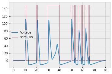
Problem 51-1
Location: Overleaf for explanations; assignment-problems/binary_search.py for code
a. (2 points) Write a function binary_search(entry, sorted_list) that finds an index of entry in the sorted_list. You should do this by repeatedly checking the midpoint of the list, and then recursing on the lower or upper half of the list as appropriate. (If there is no midpoint, then round up or round down consistently.)
Assert that your function passes the following test:
>>> binary_search(7, [2, 3, 5, 7, 8, 9, 10, 11, 13, 14, 15, 16])
3
b. (1 points) Suppose you have a sorted list of 16 elements. What is the greatest number of iterations of binary search that would be needed to find the index of any particular element in the list? Justify your answer.
c. (2 points) State and justify a recurrence equation for the time complexity of binary search on a list of $n$ elements. Then, use it to derive the time complexity of binary search on a list of $n$ elements.
Problem 51-2
Grading: 5 points
In CombatEngine, write a method generate_combat_array() that returns an array of combat states:
[
    {'location': (1,2),
    'order': [{'player': 1, 'unit': 0,},
              {'player': 0, 'unit': 1},
              {'player': 1, 'unit': 1}],
    },
    {'location': (5,10),
    'order': [{'player': 0, 'unit': 0},
              {'player': 1, 'unit': 2},
              {'player': 1, 'unit': 4}],
    },
],
Problem 51-3
Location: Overleaf
Grading: 20 points for a complete draft that is factually correct with proper grammar and usage of transitions / paragraphs, along with descriptions of several images and code snippets to be included in your post.
Write a first draft of your blog post. If you have any images / code snippets in mind, you can just describe them verbally, as follows. We'll fill in images and code later.
Here is an example snippet:
...

To squash the possible outputs into the interval [0,1], we
need to use a sigmoid function of the form

$$y = \dfrac{1}{1+e^{\beta x}}.$$

[image: graph of sigmoidal data with a sigmoid function
running through it]

When we wish to fit the logistic regression for multiple input
variables, we can replace the exponent with a linear combination
of features:

$$y = \dfrac{1}{1+e^{\beta_0 + \beta_1 x_1 + \beta_2 x_2 + \cdots + \beta_n x_n}}.$$

The sigmoid function is nonlinear, so it may seem that we
need to take a different approach to fitting the logistic
regression. Howerver, using a bit of algebra, we can transform the
logistic regression problem into a linear regression problem:

\begin{align*}
y &= \dfrac{1}{1+e^{\beta_0 + \beta_1 x_1 + \beta_2 x_2 + \cdots + \beta_n x_n}} \\
1+e^{\beta_0 + \beta_1 x_1 + \beta_2 x_2 + \cdots + \beta_n x_n} &= \dfrac{1}{y} \\
e^{\beta_0 + \beta_1 x_1 + \beta_2 x_2 + \cdots + \beta_n x_n} &= \dfrac{1}{y} - 1 \\
\beta_0 + \beta_1 x_1 + \beta_2 x_2 + \cdots + \beta_n x_n &= \ln \left( \dfrac{1}{y} - 1 \right) \\
\end{align*}

So, if we transform the $y$-values of the dataset as

$$y \to \ln \left( \dfrac{1}{y} - 1 \right),$$

then the logistic regression problem reduces to a linear regression
problem using the transformed $y$-values. To obtain our logistic
regression coefficients, we transform $y$ and fit the linear regression
as follows:

[code: transform y, fit linear regression]

...
We're shooting for something in the style of Hacker News posts. Here are some examples of the kind of style that we're looking for:
- https://karpathy.github.io/2016/05/31/rl/
- https://medium.com/gradientcrescent/fundamentals-of-reinforcement-learning-automating-pong-in-using-a-policy-model-an-implementation-b71f64c158ff
- https://colah.github.io/posts/2015-08-Backprop/
George: Linear and Logistic Regression, Part 1: Understanding the Models
What is "regression", and why do we care about it?
In particular, what are linear and logistic regression? What "shape" of data do they model, what is the mathematical form for each of them? (Don't explain how to actually fit the model. This will be done by Colby in part 2.)
Give some examples of situations in which you'd use linear regression instead of logistic regression. Then, give some examples of situations in which you'd use logistic regression instead of linear regression. Make sure you explain why you'd use one model instead of the other.
Explain how in particular, logistic regression can be used to model probability. Give some examples of probabilities that we might model using logistic regression. Why can't we use linear regression to model probability?
Explain how a logistic regression model can be adjusted to model variables that range from 0 to some maximum other than 1. Give a couple examples of situations in which we'd want to do this (e.g. ratings on a scale of 0-10).
Explain how a logistic model can be adjusted to model variables that range from some general lower bound $a$ to some general upper bound $b.$ Give a couple examples of situations in which we'd want to do this.
Colby: Linear and Logistic Regression, Part 2: Fitting the Models
Briefly recap: what "shape" of data do linear and logistic regression model, and what are their mathematical forms?
How do you fit a linear regression model using matrix algebra? What is the pseudoinverse, and why is it needed? Talk through the general method, and illustrate on a concrete example.
How do you fit a logistic regression model using matrix algebra? Talk through the general method, and illustrate on a concrete example.
How is logistic regression related to linear regression? (Logistic regression is really just linear regression on a transformation of variables.)
Explain how you made LogisticRegressor really compact by having it inherit from LinearRegressor. Include a Python code snippet.
Riley: Linear and Logistic Regression, Part 3: Categorical Variables, Interaction Terms, and Nonlinear Transformations of Variables
What if you want to model a dataset using linear or logistic regression, but it has categorical variables? Give a couple examples of situations in which this might happen.
In order to model the dataset, what do you have to do to the categorical variables, and why?
What are "interactions" between variables? Give a couple examples of situations when you might need to incorporate interactions into the models.
As-is, can linear or logistic regression capture interactions between variables? Why not? Explain some bad things that might happen if you use vanilla linear or logistic regression in a case when it's important to capture interactions between variables.
What do you have to do to the dataset in order to for your linear or logistic regression to capture interactions?
You can transform the dataset in any way before fitting a linear regression. Consequently, you can actually model many types of nonlinear data by reducing the task down to a linear regression. For example, you can fit a polynomial model using linear regression. Give an example scenario of when you might want to do this. How can you do this?
Logistic regression reduces to linear regression. Polynomial regression reduces to linear regression. Is there any type of regression model that you can't just reduce down to a linear regression? How can you tell whether or not a regression model can be reduced to linear regression?
David: Predator-Prey Modeling with Euler Estimation
What is a predator-prey relationship? Give several concrete examples.
How can we model a predator-prey relationship using differential equations? How do you set up the system of differential equations, and why do you set the system up that way?
What is Euler estimation, and how can you use it to plot the approximate solution to systems of differential equations? Write some code.
How do you choose your step size? What bad thing happens if you choose a step size that is too big? What bad thing happens if you choose a really really really small step size?
Why do oscillations arise in the plot? What do they actually represent in terms of the predator and prey?
Elijah: Solving Magic Squares using Backtracking
What is a magic square? Talk about it in general, not just the 3x3 case. This link will be helpful: https://mathworld.wolfram.com/MagicSquare.html
How can you solve a magic square using brute-force search? Write some code.
What's the problem with brute-force search? Run some actual simulations to see how long it takes you to find a solution to a 3x3 magic square using brute force. Then try the 4x4, 5x5, etc and make a graph. State the results as something ridiculous -- e.g. (it'll take me years to solve a something-by-something magic square)
What is the most obvious inefficiency in brute-force search? (It spends a lot of time exploring invalid combinations.)
How can you overcome this inefficiency using "backtracking", i.e. intelligent search? https://en.wikipedia.org/wiki/Sudoku_solving_algorithms#Backtracking
Write some code for how to implement backtracking using a bunch of nested for loops (i.e. the ugly solution). Run some actual simulations to see how long it takes you to find a solution to a 3x3 magic square using backtracking. Then try the 4x4, 5x5, etc and make a graph.
How can you write the code more compactly using a single while loop?
Problem 50-1
Location: Overleaf
Grading: 7 points
Suppose a magician does a trick where they show you a die that has 6 sides labeled with the numbers $1$ through $6.$ Then, they start rolling the die, and they roll two $1$s and three $2$s. You suspect that they might have switched out the die for a "trick" die that is labeled with three sides of $1$ and three sides of $2.$
Let $\text{switch}$ be the event that the magician actually switched out the die.
PART 0
Given the data, compute the likelihood $P(\text{two rolls of 1 and three rolls of 2} \, | \, \text{switch}).$ Your work should lead to the following result: $$ P(\text{two rolls of 1 and three rolls of 2} \, | \, \text{switch}) = \begin{cases} 0.3125, \quad \textrm{switch = True} \\ 0.001286, \quad \textrm{switch = False} \\ \end{cases}$$
- Hint: you'll need to use combinations.
PART 1
Suppose that, before the magician rolled the die, you were agnostic: you believed there was a $50\%$ chance that the die was fair (i.e. a $50\%$ chance that the die was switched out for a biased one).
a. Given your prior belief, what is the prior distribution $P(\text{switch})?$
$$ P(\textrm{switch}) = \begin{cases} \_\_\_, \quad \textrm{switch = True} \\ \_\_\_, \quad \textrm{switch = False} \\ \end{cases}$$b. What is the posterior distribution $P(\text{switch} \, | \, \text{two rolls of 1 and three rolls of 2})?$ Your work should lead to the following result: $$ P(\text{switch} \, | \, \text{two rolls of 1 and three rolls of 2}) = \begin{cases} 0.996, \quad \textrm{switch = True} \\ 0.004, \quad \textrm{switch = False} \\ \end{cases}$$
PART 2
Suppose that, before the magician rolled the die, you were optimistic: you believed there was a $99\%$ chance that the die was fair (i.e. a $1\%$ chance that the die was switched out for a biased one).
a. Given your prior belief, what is the prior distribution $P(\text{switch})?$
$$ P(\textrm{switch}) = \begin{cases} \_\_\_, \quad \textrm{switch = True} \\ \_\_\_, \quad \textrm{switch = False} \\ \end{cases}$$b. What is the posterior distribution $P(\text{switch} \, | \, \text{two rolls of 1 and three rolls of 2})?$ Your work should lead to the following result: $$ P(\text{switch} \, | \, \text{two rolls of 1 and three rolls of 2}) = \begin{cases} 0.711, \quad \textrm{switch = True} \\ 0.289, \quad \textrm{switch = False} \\ \end{cases}$$
PART 3
Suppose that, before the magician rolled the die, you were pessimistic: you believed there was a $1\%$ chance that the die was fair (i.e. a $99\%$ chance that the die was switched out for a biased one).
a. Given your prior belief, what is the prior distribution $P(\text{switch})?$
$$ P(\textrm{switch}) = \begin{cases} \_\_\_, \quad \textrm{switch = True} \\ \_\_\_, \quad \textrm{switch = False} \\ \end{cases}$$b. What is the posterior distribution $P(\text{switch} \, | \, \text{two rolls of 1 and three rolls of 2})?$ Your work should lead to the following result: $$ P(\text{switch} \, | \, \text{two rolls of 1 and three rolls of 2}) = \begin{cases} 0.99996, \quad \textrm{switch = True} \\ 0.00004, \quad \textrm{switch = False} \\ \end{cases}$$
Problem 50-2
Location: Overleaf
Grading: 7 points
One of the simplest ways to model the spread of disease using differential equations is the SIR model. The SIR model assumes three sub-populations: susceptible, infected, and recovered.
The number of susceptible people $(S)$ decreases at a rate proportional to the rate of meeting between susceptible and infected people (because susceptible people have a chance of catching the disease when they come in contact with infected people).
The number of infected people $(I)$ increases at a rate proportional to the rate of meeting between susceptible and infected people (because susceptible people become infected after catching the disease), and decreases at a rate proportional to the number of infected people (as the diseased people recover).
The number of recovered people $(R)$ increases at a rate proportional to the number of infected people (as the diseased people recover).
a. Write a system of differential equations to model the system.
$$\begin{cases} \dfrac{\textrm{d}S}{\textrm{d}t} &= \_\_\_, \quad S(0) = \_\_\_ \\ \dfrac{\textrm{d}I}{\textrm{d}t} &= \_\_\_, \quad I(0) = \_\_\_ \\ \dfrac{\textrm{d}R}{\textrm{d}t} &= \_\_\_, \quad R(0) = \_\_\_ \end{cases}$$Make the following assumptions:
There are initially $1000$ susceptible people and $1$ infected person.
The number of meetings between susceptible and infected people each day is proportional to the product of the numbers of susceptible and infected people, by a factor of $0.01 \, .$ The transmission rate of the disease is $3\%.$ (In other words, $3\%$ of meetings result in transmission.)
Each day, $2\%$ of infected people recover.
Check: If you've written the system correctly, then at $t=0,$ you should have
$$ \dfrac{\textrm{d}S}{\textrm{d}t} = -0.3, \quad \dfrac{\textrm{d}I}{\textrm{d}t} = 0.3, \quad \dfrac{\textrm{d}R}{\textrm{d}t} = 0.2 \, . $$b. Plot the system and include the plot in your Overleaf document. (You get to choose your own step size and interval. Choose a step size small enough that the model doesn't blow up, but large enough that the simulation doesn't take long to run. Choose an interval that displays all the main features of the differential equation -- you'll see what I mean if you play around with various plotting intervals.)
c. Explain what the plot shows, and explain why this happens.
Problem 50-3
Location: space-empires/src/game.py generate_state()
Grading: 7 points
Refactor your game state generator to use the structure shown below. Print out your game state at each moment in your DumbPlayer tests. (In the next assignment, we will refactor the tests to actually use the game state, but for now, just print it out.)
game_state = {
    'turn': 4,
    'phase': 'Combat', # Can be 'Movement', 'Economic', or 'Combat'
    'round': None, # if the phase is movement, then round is 1, 2, or 3
    'player_whose_turn': 0, # index of player whose turn it is (or whose ship is attacking during battle),
    'winner': None,
    'players': [
        {'cp': 9
        'units': [
            {'location': (5,10),
            'type': Scout,
            'hits': 0,
            'technology': {
                'attack': 1,
                'defense': 0,
                'movement': 3
            }},
            {'location': (1,2),
            'type': Destroyer,
            'hits': 0,
            'technology': {
                'attack': 0,
                'defense': 0,
                'movement': 2
            }},
            {'location': (6,0),
            'type': Homeworld,
            'hits': 0,
            'turn_created': 0
            },
            {'location': (5,3),
            'type': Colony,
            'hits': 0,
            'turn created': 2
            }],
        'technology': {'attack': 1, 'defense': 0, 'movement': 3, 'ship size': 0}
    },
    {'cp': 15
        'units': [
        {'location': (1,2),
        'type': Battlecruiser,
        'hits': 1,
        'technology': {
            'attack': 0,
            'defense': 0,
            'movement': 0
        }},
        {'location': (1,2),
        'type': Scout,
        'hits': 0,
        'technology': {
            'attack': 1,
            'defense': 0,
            'movement': 0
        }},
        {'location': (5,10),
        'type': Scout,
        'hits': 0,
        'technology': {
            'attack': 1,
            'defense': 0,
            'movement': 0
        }},
        {'location': (6,12),
        'type': Homeworld,
        'hits': 0,
        'turn_created': 0
        },
        {'location': (5,10),
        'type': Colony,
        'turn created': 1
        }],
        'technology': {'attack': 1, 'defense': 0, 'movement': 0, 'ship size': 0}
    }],
    'planets': [(5,3), (5,10), (1,2), (4,8), (9,1)]
}
Problem 49-1
Location: Overleaf
Grading: 11 points total
a. (1 point) Given that $X \sim p(x),$ where $p(x)$ is a continuous distribution, prove that for any real number $a$ we have $E[aX] = aE[X].$
- You should start by writing $E[aX]$ as an integral, manipulating it, and then simplifying the result into $aE[X].$ The manipulation will just be 1 step.
b. (1 point) Given that $X_1, X_2 \sim p(x),$ where $p(x)$ is a continuous distribution, prove that $E[X_1 + X_2] = E[X_1] + E[X_2].$
- You should start by writing $E[X_1 + X_2]$ as an integral, manipulating it, and then simplifying the result into $E[X_1] + E[X_2].$ The manipulation will just be 1 step.
c. (3 points) Given that $X \sim p(x)$ where $p(x)$ is a continuous probability distribution, prove the identity $\text{Var}[X] = E[X^2] - E[X]^2.$
- You should start by writing $\text{Var}[X]$ as an integral, expanding it out, into multiple integrals, and then simplifying the result into $E[X^2] - E[X]^2.$ The manipulation will involve several steps.
d. (3 points) Use bisection search to estimate $\sqrt{5}$ to $4$ decimal places by hand, showing your work at each step of the way. See problem 5-2 for a refresher on bisection search.
e. (3 points) Use "merge sort" to sort the list [4,8,7,7,4,2,3,1]. Do the problem by hand and show your work at each step of the way. See problem 23-2 for a refresher on merge sort.
Problem 49-2
We've been doing a lot of likelihood estimation. However, we've been hand-waving the fact that the likelihood actually represents the correct probability distribution of a parameter once we normalize it.
The mathematical reason why the normalized likelihood actually represents the correct probability distribution is Bayes' theorem. Bayes' theorem states that for any two events $A$ and $B,$ if $B,$ occurred, then the probability of $A$ occurring is
$$\begin{align} P(A \, | \, B) = \dfrac{P(A \text{ and } B)}{P(B)}. \end{align}$$Note that Bayes' theorem comes from the "multiplication law" for conditional probability:
$$\begin{align} P(A \text{ and } B) = P(A \, | \, B)P(B). \end{align}$$In most of our contexts, we're interested in the probability of a parameter taking a particular value, given some observed data. So, using Bayes' theorem and the multiplication law, we have
$$\begin{align*} P(\text{parameter}=k \, | \, \text{data}) &= \dfrac{P(\text{parameter}=k \text{ and data})}{P(\text{data})} \\ &= \dfrac{P(\text{data} \, | \, \text{parameter}=k) P(\text{parameter}=k)}{P(\text{data})}. \end{align*}$$Now, $P(\text{data})$ is just a constant, so we have
$$\begin{align*} P(\text{parameter}=k \, | \, \text{data}) &= \dfrac{P(\text{data} \, | \, \text{parameter}=k) P(\text{parameter}=k)}{\text{some constant}} \\ &\propto P(\text{data} \, | \, \text{parameter}=k) P(\text{parameter}=k) \end{align*}$$where the "$\propto$" symbol means "proportional to".
The term $P(\text{parameter}=k)$ is called the prior distribution and represents the information that we know about the parameter before we have observed the data. If we haven't observed any data, we often take this prior distribution to be the uniform distribution.
The term $P(\text{data} \, | \, \text{parameter}=k)$ is the probability of observing the data, given that the parameter is $k.$ This is equivalent to the likelihood of the parameter $k,$ given the data.
The term $P(\text{parameter}=k \, | \, \text{data})$ is called the posterior distribution and represents the information that we know about the parameter after we have observed the data.
In all the problems that we have done until now, we have taken the prior distribution to be the uniform distribution, meaning that we don't know anything about the parameter until we have gathered some data. Since the uniform distribution is constant, we have
$$\begin{align*} P(\text{parameter}=k \, | \, \text{data}) &\propto P(\text{data} \, | \, \text{parameter}=k) P(\text{parameter}=k) \\ &\propto P(\text{data} \, | \, \text{parameter}=k) (\text{some constant}) \\ &\propto P(\text{data} \, | \, \text{parameter}=k). \end{align*}$$Remember that $P(\text{data} \, | \, \text{parameter}=k)$ is just the likelihood, $\mathcal{L}(\text{parameter}=k \, | \, \text{data}),$ so we have
$$\begin{align*} P(\text{parameter}=k \, | \, \text{data}) \propto \mathcal{L}(\text{parameter}=k \, | \, \text{data}). \end{align*}$$And there we go! The distribution of the parameter is proportional to the likelihood.
THE ACTUAL QUESTION BEGINS HERE...
Grading: 13 points possible
Location: Overleaf
Suppose a wormhole opens and people begin testing it out for travel purposes. You want to use the wormhole too, but you're not sure whether it's safe. Some other people don't seem to care whether it's safe, so you decide to count the number of successful travels by others until you're $99\%$ sure the risk of disappearing forever into the wormhole is no more than your risk of dying from a car crash in a given year ($1$ in $10\,000$).
You model the situation as $P(\text{success}) = k$ and $P(\text{failure}) = 1-k.$ "Success" means successfully entering and successfully exiting the wormhole, while "failure" means entering but failing to exit the wormhole.
PART 1 (Bayesian inference with a uniform prior)
Start by assuming a uniform prior distribution (i.e. you know nothing about $k$ until you've collected some data). So, $k$ initially follows the uniform distribution over the interval $[0,1]\mathbin{:}$
$$P(k) = \dfrac{1}{1-0} = 1, \quad k \in [0,1]$$a. (1 point) Other people make $1\,000$ successful trips through the wormhole with no failures. What is the likelihood function for $k$ given these $1\,000$ successful trips?
- Check that your function is correct by verifying a particular input/output pair: when you plug in $k=0.99,$ you should get $\mathcal{L}(k=0.99 \, | \, 1\,000 \text{ successes}) = 0.000043$ (rounded to 6 decimal places).
b. (1 point) What is the posterior distribution for $k$ given these $1\,000$ successful trips? (This is the same as just normalizing the likelihood function).
- Check that your function is correct by verifying a particular input/output pair: when you plug in $k=0.99,$ you should get $p(k=0.99 \, | \, 1\,000 \text{ successes}) = 0.043214$ (rounded to 6 decimal places).
c. (2 points) Assuming that you will use the wormhole $500$ times per year, what is the posterior probability that the risk of disappearing forever into the wormhole is no more than your risk of dying from a car crash in a given year ($1$ in $10\,000$)? In other words, what is $P \left( 1-k^{500} \leq \dfrac{1}{10\,000} \, \Bigg| \, 1\,000 \text{ successes} \right)?$
- Note that $k^{500}$ represents the probability of $500$ successes in a row, so $1-k^{500}$ represents the probability of at least one failure over the course of $500$ trips through the wormhole.
- Check your answer: you should get $0.000200$ (rounded to 4 decimal places)
PART 2 (Updating by inspecting the posterior)
You keep on collecting data until your posterior distribution is $P(k \, | \, \text{? successes}) = 5\,001 k^{5\,000}.$ But then you forget how many successes you have counted. Because this is a rather simple scenario, it's easy to find this number by inspecting your posterior distribution.
a. (1 point) Looking at the given posterior distribution, how many successes have you counted?
b. (2 points) Suppose you observe $2\,000$ more successes. What is the posterior distribution now?
- Check that your function is correct by verifying a particular input/output pair: when you plug $k=0.999$ into your posterior distribution, you should get $P(k=0.999 \, | \, 2\,000 \text{ more successes}) = 6.362$ (rounded to 3 decimal places).
PART 3 (Bayesian updating)
To get some practice with the general procedure of Bayesian inference with a non-uniform prior, let's re-do Part 2, supposing you weren't able to remember the number of successes by inspecting your posterior distribution.
This time, you'll use $P(k \, | \, \text{? successes}) = 5\,001 k^{5\,000}$ as your prior distribution.
a. (3 points) Suppose you observe $2\,000$ more successes. Fill in the blanks: $$\begin{align*} \text{prior distribution: }& P(k) = 5\,001 k^{5\,000} \\ \text{likelihood: }& P(2\,000 \text{ more successes} \, | \, k) = \_\_\_ \\ \text{prior } \times \text{likelihood: }& P(2\,000 \text{ more successes} \, | \, k)P(k) = \_\_\_ \\ \text{posterior distribution: } & P(k \, | \, 2\,000 \text{ more successes}) = \_\_\_ \end{align*}$$
- Check that your function is correct by verifying a particular input/output pair: when you plug in $k=0.999$ to your likelihood, you should $P(2\,000 \text{ more successes} \, | \, k = 0.999) = 0.1351$ (rounded to 4 decimal places)
- Your posterior distribution should come out exactly the same as in 2b, and you need to show the work for why this happens.
PART 4 (Inference)
Let's go back to the moment when you forgot the number of successes, and your posterior distribution was is $P(k \, | \, \text{? successes}) = 5\,001 k^{5\,000}.$
a. (3 points) Assuming that you will use the wormhole $500$ times per year, how many more people do you need to observe successfully come out of the wormhole to be $99\%$ sure the risk of disappearing forever into the wormhole is no more than your risk of dying from a car crash in a given year ($1$ in $10\,000$)?
- In other words, find the least $N$ such that $P\left(1-k^{500} \leq \dfrac{1}{10\,000} \, \Bigg| \, N \text{ more successes} \right) = 0.99 \, .$
- Check that your function is correct by verifying a particular input/output pair: your answer should come out to $N = 23 \, 019 \, 699.$
Problem 49-3
If your EulerEstimator is not currently working, then fix it. Make sure to write a post if you run into any issues you're not able to solve.
Problem 48-1
Location: Write your answers in LaTeX on Overleaf.com using this template.
Suppose that you wish to model a deer population $D(t)$ and a wolf population $W(t)$ over time $t$ (where time is measured in years).
Initially, there are $100$ deer and $10$ wolves.
In the absence of wolves, the deer population would increase at the instantaneous rate of $60\%$ per year.
In the absence of deer, the wolf population would decrease at the instantaneous rate of $90\%$ per year.
The wolves and deer meet at a rate of $0.1$ times per wolf per deer per year, and every time a wolf meets a deer, it has a $50\%$ chance of successfully killing and eating the deer. In other words, the deer population decreases at a rate of $0.1$ deer per deer killed per year.
The rate at which the wolf population increases is proportional to the number of deer that are killed, by a factor of $0.4.$ In other words, the wolf population grows by a rate of $0.4$ wolves per deer killed per year.
a. (2 points) Set up a system of differential equations to model the situation:
\begin{cases} \dfrac{\text{d}D}{\textrm{d}t} = (\_\_\_) D + (\_\_\_) DW, \quad D(0) = \_\_\_ \\ \dfrac{\text{d}W}{\textrm{d}t} = (\_\_\_) W + (\_\_\_) DW, \quad W(0) = \_\_\_ \\ \end{cases}Check your answer: at $t=0,$ you should have $\dfrac{\text{d}D}{\textrm{d}t} = 10$ and $\dfrac{\text{d}W}{\textrm{d}t} = 11.$
Here's some latex for you to use:
$$\begin{cases}
\dfrac{\text{d}D}{\textrm{d}t} = (\_\_\_) D + (\_\_\_) DW, \quad D(0) = \_\_\_ \\
\dfrac{\text{d}W}{\textrm{d}t} = (\_\_\_) W + (\_\_\_) DW, \quad W(0) = \_\_\_ \\
\end{cases}$$
b. (2 points) Plot the system of differential equations for $0 \leq t \leq 100,$ using a step size $\Delta t = 0.001.$ Then, download your plot and put it in your writeup. (I updated the latex template to show to include an example of inserting an image.)
c. (2 points) In the plot, you should see oscillations. What does this mean in terms of the wolf and deer populations? Why does this happen?
def f(x):
    return g(x)

def g(x):
    return 0

f(0)
Problem 48-2
a. (2 points) Refactor your Player class so that a player is initialized with a strategy class, and the strategy class is stored within player.strategy.
b. (4 points) In Game, create a method generate_state() that looks at the game board, players, units, etc and puts all the relevant information into a nested "state" dictionary. In the next class, we will come to an agreement about how this "state" dictionary should be structured, but for now, I want everyone to give it a shot and we'll see what we come up with.
Note: DON'T do this now, but just to let you know what's coming -- once we've come to an agreement regarding the structure of the "state" dictionary, you will be doing the following:
Rename
dumb_player.pytodeprecated_dumb_player.py, renamecombat_player.pytodeprecated_combat_player.py, and renameyourname_strategy_player.pytodeprecated_yourname_strategy_player.py.Write classes
DumbStrategy,CombatStrategy, andYourNameStrategythat each contain the strategies for following methods:will_colonize_planet(colony_ship, game_state): returns eitherTrueorFalse; will be called whenever a player's colony ship lands on an uncolonized planetdecide_ship_movement(ship, game_state): returns the coordinates to which the player wishes to move their ship.decide_purchases(game_state): returns a list of ship and/or technology types that you want to purchase; will be called during each economic round.decide_removals(game_state): returns a list of ships that you want to remove; will be called during any economic round when your total maintenance cost exceeds your CP.decide_which_ship_to_attack(attacking_ship, game_state): looks at the ships in the combat order and decides which to attack; will be called whenever it's your turn to attack
Make sure your tests work when you use players with
DumbStrategyorCombatStrategyRun a game with
YourNameStrategyvsDumbStrategyand ensure that your strategy beats the dumb strategy.
Problem 48-3
Soon, a part of your homework will consist of writing up blog posts about things you've done. I've come up with 11 topics so far and put them in a spreadsheet. Each person is going to write about a different topic. So I'm going to try to match up everyone with topics they're most interested in. Take a look at this spreadsheet and rank your top 5 posts in order of preference (with 1 being the most preferable, 2 being the next-most preferable, and so on).
We're doing this because we need to build up some luck surface area. It's great that we're doing so much cool stuff, but part of the process of opening doors is telling people what you're doing. Writing posts is a way to do that. And it's also going to help contribute to developing your portfolios, so that you have evidence of what you're doing.
Problem 47-1
Location: Write your answers in LaTeX on Overleaf.com using this template.
Grading: 2 points per part
Several witnesses reported seeing a UFO during the following time intervals:
$$ \text{data}=\bigg\{ [12,13], \, [12,13.5], \, [14,15], \, [14,16] \bigg\} $$The times represent hours in military time:
- $12$ is noon,
- $13$ is 1 pm,
- $13.5$ is 1:30 pm,
- ...
Suppose you want to quantify your certainty regarding when the UFO arrived and when it left.
Assume the data came from $\mathcal{U}[a,b],$ the uniform distribution on the interval $[a,b].$ This means the UFO arrived at time $a$ and left at time $b.$
Watch out! The data do NOT correspond to samples of $[a,b].$ Rather, the data correspond to subintervals of $[a,b].$
a. Compute the likelihood function $\mathcal{L}([a,b]\,|\,\text{data}).$
Your result should come out to $\dfrac{3}{(b-a)^4}.$
Hint: if the UFO was there from $t=a$ to $t=b,$ then what's the probability that a single random observation of the UFO would take place between 12:00 and 13:30? In other words, if you had to choose a random number between $a$ and $b,$ what's the probability that your random number would be between $12$ and $13.5?$
b. Normalize the likelihood function so that it can be interpreted as a probability density.
As an intermediate step to solve for the constant of normalization, you will have to take a double integral $\displaystyle \int_{b_\text{min}}^{b_\text{max}} \int_{a_\text{min}}^{a_\text{max}} \mathcal{L}([a,b]\,|\,\text{data}) \, \text{d}a \, \text{d}b$. Two of the bounds will be infinite, and two of the bounds will be finite.
To figure out the appropriate intervals of integration for $a,b,$ ask yourself the following:
What is the highest possible value for $a$ (i.e. the latest the UFO could have arrived) given the data?
What is the lowest possible value for $b$ (i.e. the earliest the UFO could have left) given the data?
c. What is the probability that the UFO came and left sometime during the day that it was sighted? In other words, what is the probability that $0<a<a_\text{max}$ and $b_\text{min} < b < 24?$
- Your answer should come out to $\frac{41}{48}.$
d. What is the probability that the UFO arrived before 10am?
- Your answer should come out to $\frac{4}{9}.$
Problem 47-2
Begin implementing your custom strategy player as a class (YourName)StrategyPlayer. In this assignment, you will write pseudocode for the components of your strategy related to movement. Again, assume a $13 \times 13$ board.
By "pseudocode", I mean that you should still write a class and use Python syntax, but your player doesn't actually have to "work" when you run the code. You just need to translate your strategy ideas into a sketch of what it would ideally look like if you coded it up.
For example, if your colonization strategy is to colonize a planet only if it is at least $2$ spaces away from a planet that you have already colonized, then the following "pseudocode" would be fine, even if (for example) you haven't actually implemented
other_planet.colonizer_player_number.
def calc_distance(coords_1, coords_2):
    x_1, y_1 = coords_1
    x_2, y_2 = coords_2
    return abs(x_2 - x_1) + abs(y_2 - y_1)

def will_colonize_planet(colony_ship, planet, game):
    for other_planet in game.board.planets:
        if other_planet.colonizer_player_number == self.player_number:
            distance = self.calc_distance(planet.coordinates, other_planet.coordinates)
            if distance < 2:
                return False
    return True
a. (2 points) Implement your colonization logic within the method Player.will_colonize_planet(colony_ship, planet, game) that returns either True or False.
This function will be called whenever a player's colony ship lands on an uncolonized planet.
When we integrate this class into the game (you don't have to do it yet), the game will ask the player whether it wants to colonize a particular planet, and the player will use the
gamedata to determine whether it wants to colonize.
b. (6 points) Implement your movement logic within the method Player.decide_ship_movement(ship, game) that returns the coordinates to which the player wishes to move their ship.
- When we integrate this class into the game (you don't have to do it yet), the game will ask the player where it wants to move to, and the player will use the
gamedata to make a decision.
Problem 46-1
Location: machine-learning/analysis/signal_separation.py
Grading: 6 points total
Use your DataFrame and LinearRegressor to solve the following regression problems.
PART A (2 points)
The following dataset takes the form $$y = a + bx + cx^2 + dx^3$$ for some constants $a,b,c,d.$ Use linear regression to determine the best-fit values of $a,b,c,d.$
[(0.0, 4.0),
 (0.2, 8.9),
 (0.4, 17.2),
 (0.6, 28.3),
 (0.8, 41.6),
 (1.0, 56.5),
 (1.2, 72.4),
 (1.4, 88.7),
 (1.6, 104.8),
 (1.8, 120.1),
 (2.0, 134.0),
 (2.2, 145.9),
 (2.4, 155.2),
 (2.6, 161.3),
 (2.8, 163.6),
 (3.0, 161.5),
 (3.2, 154.4),
 (3.4, 141.7),
 (3.6, 122.8),
 (3.8, 97.1),
 (4.0, 64.0),
 (4.2, 22.9),
 (4.4, -26.8),
 (4.6, -85.7),
 (4.8, -154.4)]
PART B (4 points)
The following dataset takes the form $$y = a \sin(x) + b \cos(x) + c \sin(2x) + d \cos(2x)$$ for some constants $a,b,c,d.$ Use linear regression to determine the best-fit values of $a,b,c,d.$
[(0.0, 7.0),
 (0.2, 5.6),
 (0.4, 3.56),
 (0.6, 1.23),
 (0.8, -1.03),
 (1.0, -2.89),
 (1.2, -4.06),
 (1.4, -4.39),
 (1.6, -3.88),
 (1.8, -2.64),
 (2.0, -0.92),
 (2.2, 0.95),
 (2.4, 2.63),
 (2.6, 3.79),
 (2.8, 4.22),
 (3.0, 3.8),
 (3.2, 2.56),
 (3.4, 0.68),
 (3.6, -1.58),
 (3.8, -3.84),
 (4.0, -5.76),
 (4.2, -7.01),
 (4.4, -7.38),
 (4.6, -6.76),
 (4.8, -5.22)]
Problem 46-2
Grading: 8 points total
Location: Write your answers in LaTeX on Overleaf.com using this template.
PART A (2 points per part)
The following statements are false. For each statement, explain why it is false, and give a concrete counterexample that illustrates that it is false.
To compute the expected values of all the variables $(x_1, x_2, \ldots, x_n),$ that follow a joint distribution $p(x_1, x_2, \ldots, x_n),$ you need to compute the equivalent of $n$ integrals (assuming that a double integral is the equivalent of $2$ integrals, a triple integral is the equivalent of $3$ integrals, and so on).
If $p(x)$ is a valid probability distribution, and we create a function $f(x,y) = p(x),$ then $f(x,y)$ is a valid joint distribution.
PART B (4 points)
The following statement is true. First, give a concrete example on which the statement holds true. Then, construct a thorough proof.
- If $f(x)$ and $g(y)$ are valid probability distributions, and we create a function $h(x,y) = f(x)g(y),$ then $h(x,y)$ is a valid probability distribution.
Problem 46-3
Grading: 10 points total (2 points for each strategy description + justification)
Location: Write your answers in LaTeX on Overleaf.com using this template.
Write up specifications for your own custom strategy player.
Make the specifications simple enough that you will be able to implement them next week without too much trouble.
Make sure that your player is able to consistently beat
DumbPlayerandCombatPlayer. But don't tailor your strategies to these opponents -- your player will battle against other classmates' players soon.
In your LaTeX doc, outline your strategy in each of the following components, and justify your reasoning for the strategy. And again, make sure it's simple enough for you to implement next week.
How will you decide where to move your ships?
How will you decide what to buy during the economic phase?
If you are unable to pay all your maintenance costs, how will you decide what ship to remove?
If you come across a planet, how will you decide whether or not to colonize it?
During battle with the enemy, when it's your ship's turn to attack an enemy ship, how will you decide which ship to attack?
Note: You can assume we're playing on a $13 \times 13$ board.
Problem 45-1
Grading: 8 points
Locations:
assignment-problems/euler_estimator.py
assignment-problems/system_plot.py
Generalize your EulerEstimator to systems of differential equations. For example, we should be able to model the system
starting at the point $\left( t, \begin{bmatrix} x_0 \\ x_1 \\ x_2 \end{bmatrix} \right) = \left( 0, \begin{bmatrix} 0 \\ 0 \\ 0 \end{bmatrix} \right)$ as follows:
>>> euler = EulerEstimator(
                derivatives = [
                    (lambda t,x: x[0] + 1),
                    (lambda t,x: x[0] + x[1]),
                    (lambda t,x: 2*x[1])
                    ],
                point = (0,(0,0,0))
            )

>>> euler.point
(0, (0, 0, 0))
>>> euler.calc_derivative_at_point()
[1, 0, 0]

>>> euler.step_forward(0.1)
>>> euler.point
(0.1, (0.1, 0, 0))

>>> euler.calc_derivative_at_point()
[1.1, 0.1, 0]
>>> euler.step_forward(-0.5)
>>> euler.point
(-0.4, (-0.45, -0.05, 0))

>>> euler.go_to_input(5, step_size = 2)

notes to help you debug:

point: (-0.4, (-0.45, -0.05, 0))
derivative: (0.55, -0.5, -0.1)
deltas: (2, (1.1, -1, -0.2))

point: (1.6, (0.65, -1.05, -0.2))
derivative: (1.65, -0.4, -2.1)
deltas: (2, (3.3, -0.8, -4.2))

point: (3.6, (3.95, -1.85, -4.4))
derivative: (4.95, 2.1, -3.7)
deltas: (1.4, (6.93, 2.94, -5.18))

>>> euler.point
(5, (10.88, 1.09, -9.58))
Also, implement plotting capability.
(continued from above tests)

>>> euler.plot([-5,5], step_size = 0.1, filename = 'plot.png')

generates three plots of x_0(t), x_1(t), and x_2(t) all
on the same axis, for t-values in the interval [-5,5]
separated by a length of step_size
Once you've got a plot, post it on Slack to compare with your classmates.
Problem 45-2
Grading: 3 points (1 point for fully catching up on each problem)
We'll use this assignment as a partial catch-up. If you didn't get full points on 44-1, 44-2, and 44-4, then revise and resubmit.
44-1: Make sure your final output is a fully correct magic square, meaning all the rows, columns, and diagonals (including the anti-diagonal) each add up to 15. Also, make sure your code runs quickly, meaning that you shouldn't be doing a plain brute-force search.
44-2: I've updated the problem with the correct answers so that you can verify your results. Also, you don't have to show every single little step in your work. Just show the main steps.
44-4: Make sure the game asks your player if it wants to colonize. There should be a method
will_colonize()in your player, and the game should check ifplayer.will_colonize(). For yourDumbPlayerandCombatPlayer, you can just setwill_colonize()to return false. Also, make sure yourDumbPlayertests andCombatPlayertests fully pass.
Problem 44-1
Location: assignment-problems/magic_square.py
In this problem, you will solve for all arrangements of digits $1,2,\ldots, 9$ in a $3 \times 3$ "magic square" where all the rows, columns, and diagonals add up to $15$ and no digits are repeated.
a. (4 points)
First, create a function is_valid(arr) that checks if a possibly-incomplete array is a valid magic square "so far". In order to be valid, all the rows, columns, and diagonals in an array that have been completely filled in must sum to $15.$
>>> arr1 = [[1,2,None],
           [None,3,None],
           [None,None,None]]
>>> is_valid(arr1)
True    (because no rows, columns, or diagonals are completely filled in)

>>> arr2 = [[1,2,None],
           [None,3,None],
           [None,None,4]]
>>> is_valid(arr2)
False   (because a diagonal is filled in and it doesn't sum to 15)

>>> arr3 = [[1,2,None],
           [None,3,None],
           [5,6,4]]
>>> is_valid(arr3)
False   (because a diagonal is filled in and it doesn't sum to 15)
        (it doesn't matter that the bottom row does sum to 15)

>>> arr4 = [[None,None,None],
           [None,3,None],
           [5,6,4]]
>>> is_valid(arr4)
True   (because there is one row that's filled in and it sums to 15)
b. (6 points)
Now, write a script to start filling in numbers of the array -- but whenever you reach a configuration that can no longer become a valid magic square, you should not explore that configuration any further. Once you reach a valid magic square, print it out.
- Tip: An ugly but straightforward way to solve this is to use 9 nested
forloops, along withcontinuestatements where appropriate. (Acontinuestatement allows you to immediately continue to the next item in aforloop, without executing any of the code below thecontinuestatement.)
Some of the first steps are shown below to give a concrete demonstration of the procedure:
Filling...

[[_,_,_],
 [_,_,_],
 [_,_,_]]

[[1,_,_],
 [_,_,_],
 [_,_,_]]

[[1,2,_],
 [_,_,_],
 [_,_,_]]

[[1,2,3],
 [_,_,_],
 [_,_,_]]

^ no longer can become a valid magic square

[[1,2,4],
 [_,_,_],
 [_,_,_]]

^ no longer can become a valid magic square

[[1,2,5],
 [_,_,_],
 [_,_,_]]

^ no longer can become a valid magic square

...

[[1,2,9],
 [_,_,_],
 [_,_,_]]

^ no longer can become a valid magic square

[[1,3,2],
 [_,_,_],
 [_,_,_]]

^ no longer can become a valid magic square

[[1,3,4],
 [_,_,_],
 [_,_,_]]

^ no longer can become a valid magic square

[[1,3,5],
 [_,_,_],
 [_,_,_]]

^ no longer can become a valid magic square

...

[[1,3,9],
 [_,_,_],
 [_,_,_]]

^ no longer can become a valid magic square

[[1,4,2],
 [_,_,_],
 [_,_,_]]

^ no longer can become a valid magic square

...

[[1,5,9],
 [_,_,_],
 [_,_,_]]

[[1,5,9],
 [2,_,_],
 [_,_,_]]

[[1,5,9],
 [2,3,_],
 [_,_,_]]

[[1,5,9],
 [2,3,4],
 [_,_,_]]

^ no longer can become a valid magic square

[[1,5,9],
 [2,3,5],
 [_,_,_]]

^ no longer can become a valid magic square

...
Problem 44-2
Location: Going forward, we're going to start using $\LaTeX$ for stats problems. Make an account at https://www.overleaf.com/ submit a sharable link to your document. Here is a link to an example template that you can use.
Grading: 1 point per item (8 points total)
A joint distribution is a probability distribution on two or more random variables. To work with joint distributions, you will need to use multi-dimensional integrals.
For example, given a joint distribution $p(x,y),$ the probability that $(X,Y) \in [a,b] \times [c,d]$ is given by
$$ \begin{align*} P((X,Y) \in [a,b] \times [c,d]) = \displaystyle \iint_{[a,b] \times [c,d]} p(x,y) \, \text{d}A, \end{align*} $$or equivalently,
$$ \begin{align*} P(a < X \leq b, \, c < Y \leq d) = \displaystyle \int_c^d \int_a^b p(x,y) \, \text{d}x \, \text{d}y. \end{align*} $$Part A
The joint uniform distribution $\mathcal{U}([a,b]\times[c,d])$ is a distribution such that all points $(x,y)$ have equal probability in the region $[a,b]\times[c,d]$ and zero probability elsewhere. So, it takes the form
$$p(x,y) = \begin{cases} k & (x,y) \in [a,b] \times [c,d] \\ 0 & (x,y) \not\in [a,b] \times [c,d] \end{cases}$$for some constant $k.$
i. Find the value of $k$ such that $p(x,y)$ is a valid probability distribution. Your answer should be in terms of $a,b,c,d.$
ii. Given that $(X,Y) \sim p,$ compute $\text{E}[X]$ and $\text{E}[Y].$
- Your answers should come out to $\dfrac{a+b}{2}$ and $\dfrac{c+d}{2}.$
iii. Given that $(X,Y) \sim p,$ compute $\text{Var}[X]$ and $\text{Var}[Y].$
- Your answers should come out to $\dfrac{(b-a)^2}{12}$ and $\dfrac{(d-c)^2}{12}.$
iv. Given that $(X,Y) \sim p,$ compute $P\left( (X,Y) \in \left[ \dfrac{a+3b}{4}, \dfrac{3a+b}{4} \right] \times \left[ \dfrac{2c+d}{3}, \dfrac{c+2d}{3} \right] \right).$
- Your answer should come out to $\frac{1}{6}.$
Part B
Now consider the joint exponential distribution defined by
$$p(x,y) = \begin{cases} k e^{-n x - q y} & x,y \geq 0 \\ 0 & x<0 \text{ or } y < 0 \end{cases}.$$i. Find the value of $k$ such that $p(x,y)$ is a valid probability distribution. Your answer should be in terms of $n,q.$
- Your answer should come out to $nq.$
ii. Given that $(X,Y) \sim p,$ compute $\text{E}[X]$ and $\text{E}[Y].$
- Your answers should come out to $\frac{1}{n}$ and $\frac{1}{q}.$
iii. Given that $(X,Y) \sim p,$ compute $\text{Var}[X]$ and $\text{Var}[Y].$
- Your answers should come out to $\frac{1}{n^2}$ and $\frac{1}{q^2}.$
iv. Given that $(X,Y) \sim p,$ compute $P\left( X < a, \, Y < b \right).$
- Your answer should come out to $(1-e^{-an})(1-e^{-bq}).$
Problem 44-3
Grading: 5 points
Locations:
assignment-problems/euler_estimator.py
assignment-problems/parabola_plot.py
Update EulerEstimator to make plots:
>>> euler = EulerEstimator(derivative = (lambda x: x+1),
                           point = (1,4))

>>> euler.plot([-5,5], step_size = 0.1, filename = 'plot.png')

generates a plot of the function for x-values in the
interval [-5,5] separated by a length of step_size

for this example, the plot should look like the parabola
y = 0.5x^2 + x + 2.5
Problem 44-4
a. (1 point)
Update the CP in your DumbPlayer tests. Players start with 0 CP, and the home colony generates 20 CP per round.
b. (5 points)
If you haven't already, modify your game so that whenever a colony ship moves onto a space with a planet, the game asks the player if they want to colonize. Your DumbPlayer and CombatPlayer should both choose not to colonize any planets -- but the game should ask them anyway. When you submit, include the link to the file where your game asks the players if they want to colonize, so I can verify.
c. (2 points)
Make sure your DumbPlayer and CombatPlayer tests all pass. Let's get this done once and for all so that we can move onto a manual strategy player!
Problem 43-1
Grading: 4 points for correct predictions and 4 points for code quality
Locations:
machine-learning/src/logistic_regressor.py
machine-learning/tests/test_logistic_regressor.py
If you have existing logistic regressor files and tests, rename them as follows:
machine-learning/src/deprecated_logistic_regressor.py
machine-learning/tests/test_deprecated_logistic_regressor.py
Now, create a new class LinearRegressor in machine-learning/src/logistic_regressor.py and assert that it passes the following tests. Put your tests in tests/test_logistic_regressor.py.
IMPORTANT: Your code must satisfy the following specifications:
LogisticRegressorshould inherit fromLinearRegressor.LogisticRegressorshould compute its coefficients by first replacing theprediction_columnwith the appropriate transformed values, and then fitting a linear regression.LogisticRegressorshould make a prediction by first computing the linear regression output using its coefficients, and then passing the result as input into the sigmoid function.
Note: If you have a deprecated LogisticRegressor, then you can use parts of it for inspiration, but I don't want to see any old dead code in this new class.
(continued from LinearRegressor tests...)

>>> df = df.apply('rating', lambda x: 0.1 if x==0 else x)

^ Note: a "lambda" function is a way of writing a function on a single line,
kind of like a list comprehension. The above lambda function just replaces any
values of 0 with 0.1.

>>> regressor = LogisticRegressor(df, prediction_column = 'rating', max_value = 10)

^ Note: the logistic regression model is
prediction_column = max_value / [ 1 + e^( sum of products of inputs and
                                          their corresponding multipliers ) ]

>>> regressor.multipliers
{
    'beef': -0.03900793,
    'pb': -0.02047944,
    'mayo': 1.74825378,
    'jelly': -0.39777219,
    'beef_pb': 0.14970983,
    'beef_mayo': -0.74854916,
    'beef_jelly': 0.46821312,
    'pb_mayo': 0.32958369,
    'pb_jelly': -0.5288267,
    'mayo_jelly': 2.64413352,
    'constant': 1.01248436
}

>>> regressor.predict({
    'beef': 5,
    'pb': 5,
    'mayo': 1,
    'jelly': 1,
})
0.023417479576338825

>>> regressor.predict({
    'beef': 0,
    'pb': 3,
    'mayo': 0,
    'jelly': 1,
})
7.375370259327203

>>> regressor.predict({
    'beef': 1,
    'pb': 1,
    'mayo': 1,
    'jelly': 0,
})
0.8076522077650409

>>> regressor.predict({
    'beef': 6,
    'pb': 0,
    'mayo': 1,
    'jelly': 0,
})
8.770303903540402
Problem 43-2
Grading: 0.5 points per test (6 tests total) and 3 tests for code quality. So, 6 points total.
Locations:
assignment-problems/euler_estimator.py
assignment-problems/test_euler_estimator.py
Create a class EulerEstimator in assignment-problems/euler_estimator.py that uses Euler estimation to solve a differential equation. In assignment-problems/test_euler_estimator.py, assert that the following tests pass:
>>> euler = EulerEstimator(derivative = (lambda x: x+1),
                           point = (1,4))

>>> euler.point
(1,4)
>>> euler.calc_derivative_at_point()
2     (because the derivative is f'(x)=x+1, so f'(1)=2)

>>> euler.step_forward(0.1)
>>> euler.point
(1.1, 4.2)        (because 4 + 0.1*2 = 4.2)

>>> euler.calc_derivative_at_point()
2.1
>>> euler.step_forward(-0.5)
>>> euler.point
(0.6, 3.15)        (because 4.2 + -0.5*2.1 = 3.15)

>>> euler.go_to_input(3, step_size = 0.5)

note: you should move to the x-coordinate of 3
      using a step_size of 0.5, until the final step,
      in which you need to reduce the step_size to hit 3

the following is provided to help you debug:

point, derivative, deltas
(0.6, 3.15), 1.6, (0.5, 0.8)
(1.1, 3.95), 2.1, (0.5, 1.05)
(1.6, 5), 2.6, (0.5, 1.3)
(2.1, 6.3), 3.1, (0.5, 1.55)
(2.6, 7.85), 3.6, (0.4, 1.44)

>>> euler.point
(3, 9.29)
Problem 42-1
Location: assignment-problems/poisson_distribution.txt
The Poisson distribution can be used to model how many times an event will occur within some continuous interval of time, given that occurrences of an event are independent of one another.
Its probability function is given by \begin{align*} p_\lambda(n) = \dfrac{\lambda^n e^{-\lambda}}{n!}, \quad n \in \left\{ 0, 1, 2, \ldots \right\}, \end{align*}
where $\lambda$ is the mean number of events that occur in the particular time interval.
SUPER IMPORTANT: Manipulating the Poisson distribution involves using infinite sums. However, these sums can be easily expressed using the Mclaurin series for $e^x\mathbin{:}$
\begin{align*} e^x = \sum_{n=0}^\infty \dfrac{x^n}{n!} \end{align*}PART A (1 point per correct answer with supporting work)
Consider the Poisson distribution defined by $$p_2(n) = \dfrac{2^n e^{-2}}{n!}.$$ Show that this is a valid probability distribution, i.e. all the probability sums to $1.$
Given that $N \sim p_2,$ compute $P(10 < N \leq 12).$ Write your answer in closed form, as simplified as possible (but don't expand out factorials). Pay close attention to the "less than" vs "less than or equal to" symbols.
Given that $N \sim p_2,$ compute $E[N].$ Using the Mclaurin series for $e^x,$ your answer should come out to a nice clean integer.
Given that $N \sim p_2,$ compute $\text{Var}[N].$ Using the Mclaurin series for $e^x,$ your answer should come out to a nice clean integer.
PART B (1 point per correct answer with supporting work)
Consider the general Poisson distribution defined by $$p_\lambda(n) = \dfrac{\lambda^n e^{-\lambda}}{n!}.$$ Show that this is a valid probability distribution, i.e. all the probability sums to $1.$
Given that $N \sim p_\lambda,$ compute $P(10 < N \leq 12).$ Write your answer in closed form, as simplified as possible (but don't expand out factorials).
Given that $N \sim p_\lambda,$ compute $E[N].$ Using the Mclaurin series for $e^x,$ your answer should come out really simple.
Given that $N \sim p_\lambda,$ compute $\text{Var}[N].$ Using the Mclaurin series for $e^x,$ your answer should come out really simple.
Problem 42-2
This will be a lighter assignment in case you need to catch up with the DataFrame/LinearRegressor class or the Game.
Problem 41-1
Locations: assignment-problems/assignment_41_stats.txt AND assignment-problems/assignment_41_stats.py
Grading: 1 point per part (6 points total)
In the previous assignment, you calculated the distribution of the bias of a coin by collecting some data, computing the likelihood function, and then "normalized" the likelihood function to turn it into a probability distribution.
This process is called Bayesian inference, and the probability distribution that you created using the likelihood function is called the Bayesian posterior distribution.
Later, we will learn more about the "Bayesian" in Bayesian inference, but for now, I want you to become familiar with the process. Now, you will perform another round of Bayesian inference, but this time on a different distribution.
Your friend is randomly stating positive integers that are less than some upper bound (which your friend knows, but you don't know). The numbers your friend states are as follows:
1, 17, 8, 25, 3
You assume that the numbers come from a discrete uniform distribution $U\left\{1,2,\ldots,k\right\}$ defined as follows:
$$p_k(x) = \begin{cases} \dfrac{1}{k} & x \in \left\{1,2,\ldots,k\right\} \\ 0 & x \not\in \left\{1,2,\ldots,k\right\} \end{cases}$$SHOW YOUR WORK FOR ALL PARTS OF THE QUESTION!
Compute the likelihood function $\mathcal{L}(k | \left\{ 1, 17, 8, 25, 3 \right\} ).$ Remember that the likelihood is just the probability of getting the result $ \left\{ 1, 17, 8, 25, 3 \right\}$ under the assumption that the data was sampled from the distribution $p_k(x).$ Your answer should be a piecewise function expressed in terms of $k.$
"Normalize" the likelihood function by multiplying it by some constant $c$ such that sums to $1.$ That is, find the constant $c$ such that $$\sum_{k=1}^\infty c \cdot \mathcal{L}(k | \left\{ 1, 17, 8, 25, 3 \right\}) = 1.$$ This way, we can treat $c \cdot \mathcal{L}$ as a probability distribution for $k:$ $$p(k) = c \cdot \mathcal{L}(k | \left\{ 1, 17, 8, 25, 3 \right\})$$
SUPER IMPORTANT: You won't be able to figure this out analytically (i.e. just using pen and paper). Instead, you should write a Python script inassignment-problems/assignment_41_stats.pyto approximate the sum by evaluating it for a very large number of terms. You should use as many terms as you need until the result appears to converge.What is the most probable value of $k?$ You can tell this just by looking at the distribution $p(k),$ but make sure to justify your answer with an explanation.
The largest number in the dataset is $25.$ What is the probability that $25$ is actually the upper bound chosen by your friend?
What is the probability that the upper bound is less than or equal to $30?$
Fill in the blank: you can be $95\%$ sure that the upper bound is less than $\_\_\_.$
SUPER IMPORTANT: You won't be able to figure this out analytically (i.e. just using pen and paper). Instead, you should write another Python function inassignment-problems/assignment_41_stats.pyto approximate value of $k$ needed (i.e. the number of terms needed) to have $p(K \leq k) = 0.95.$
SHOW YOUR WORK FOR ALL PARTS OF THE QUESTION!
Problem 41-2
Grading: 4 points for correct predictions and 4 points for code quality
Locations:
machine-learning/src/linear_regressor.py
machine-learning/tests/test_linear_regressor.py
machine-learning/src/logistic_regressor.py
machine-learning/tests/test_logistic_regressor.py
If you have existing linear and polynomial regressor files and tests, rename them as follows:
machine-learning/src/deprecated_linear_regressor.py
machine-learning/src/deprecated_polynomial_regressor.py
machine-learning/tests/test_deprecated_linear_regressor.py
machine-learning/tests/test_deprecated_polynomial_regressor.py
Now, create a new class LinearRegressor in machine-learning/src/linear_regressor.py and assert that it passes the following tests. Put your tests in tests/test_linear_regressor.py.
Note: You can use parts of your deprecated LinearRegressor for inspiration, but I don't want to see any old dead code in this new class.
>>> data_dict = {
    'beef': [0, 0, 0, 0, 5, 5, 5, 5, 0, 0, 0, 0, 5, 5, 5, 5],
    'pb': [0, 0, 0, 0, 0, 0, 0, 0, 5, 5, 5, 5, 5, 5, 5, 5],
    'condiments': [[],['mayo'],['jelly'],['mayo','jelly'],
                   [],['mayo'],['jelly'],['mayo','jelly'],
                   [],['mayo'],['jelly'],['mayo','jelly'],
                   [],['mayo'],['jelly'],['mayo','jelly']],
    'rating': [1, 1, 4, 0, 4, 8, 1, 0, 5, 0, 9, 0, 0, 0, 0, 0]
}
>>> df = DataFrame(data_dict, column_order = ['beef', 'pb', 'condiments'])
>>> df.columns
['beef', 'pb', 'condiments']

>>> df = df.create_all_dummy_variables()
>>> df = df.append_pairwise_interactions()
>>> df = df.append_columns({
    'constant': [1 for _ in range(len(data_dict['rating']))],
    'rating': data_dict['rating']
})
>>> df.columns
['beef', 'pb', 'mayo', 'jelly',
 'beef_pb', 'beef_mayo', 'beef_jelly', 'pb_mayo', 'pb_jelly', 'mayo_jelly'
 'constant', 'rating']

>>> linear_regressor = LinearRegressor(df, prediction_column = 'rating')
>>> linear_regressor.coefficients
{
    'beef': 0.25,
    'pb': 0.4,
    'mayo': -1.25,
    'jelly': 1.5,
    'beef_pb': -0.21,
    'beef_mayo': 1.05,
    'beef_jelly': -0.85,
    'pb_mayo': -0.65,
    'pb_jelly': 0.65,
    'mayo_jelly': -3.25,
    'constant': 2.1875
}

>>> linear_regressor.gather_all_inputs({
    'beef': 5,
    'pb': 5,
    'mayo': 1,
    'jelly': 1,
})

{
    'beef': 5,
    'pb': 5,
    'mayo': 1,
    'jelly': 1,
    'beef_pb': 25,
    'beef_mayo': 5,
    'beef_jelly': 5,
    'pb_mayo': 5,
    'pb_jelly': 5,
    'mayo_jelly': 1,
    'constant': 1
}


^ Note: this should include all interactions terms AND any constant term
that also appear in the base dataframe

>>> linear_regressor.predict({
    'beef': 5,
    'pb': 5,
    'mayo': 1,
    'jelly': 1,
})
-1.8125

>>> linear_regressor.predict({
    'beef': 0,
    'pb': 3,
    'mayo': 0,
    'jelly': 1,
})
6.8375

>>> linear_regressor.predict({
    'beef': 1,
    'pb': 1,
    'mayo': 1,
    'jelly': 0,
})
1.7775

>>> linear_regressor.predict({
    'beef': 6,
    'pb': 0,
    'mayo': 1,
    'jelly': 0,
})
8.7375
Problem 41-3
Locations: assignment-problems/assignment_41_scenarios.txt
Grading: 1 point per part (2 points total)
a. Give a real-world scenario in which something could go drastically wrong if you mistakenly use a logistic regression when the data is actually linear.
- Here's an example (which you cannot use as your answer). You're trying to predict the correct dose of a vitamin to administer to a patient. You gather a dataset of dose amount vs the vitamin concentration in the patient's blood, and you want to find the correct dose that will result in some amount of vitamin in the patient's blood. The data is linear, but you fit it with a logistic regression. As a result, because the logistic regression fits a sigmoid that "flattens out", you grossly overestimate the dose amount that is required to achieve the desired level of vitamin concentration. When you administer this overdose, the patient experiences severe vitamin overdose symptoms and possibly dies.
b. Give a real-world scenario in which something could go drastically wrong if you mistakenly use a linear regression when the data is actually sigmoid-shaped.
Problem 41-4
2 points
Get your CombatPlayer tests working. If they're working already, then congrats, you just got 2 points for free.
I'm making this worth 2 points so that there's an incentive to get this done as soon as possible (rather than just waiting to resubmit the previous assignment at some later date).
Once you get your tests working, remember to resubmit any previous assignments to get that 60% partial credit.
Problem 40-1
Location: assignment-problems/assignment_40_statistics.txt
Grading: 1 point for a correct answer to each part with all work shown.
Suppose you toss a coin $10$ times and get the result $\text{HHHHT HHHHH}.$ From this result, you estimate that the coin is biased and generally lands on heads $90\%$ of the time. But how sure can you be? Let's quantify it.
SHOW YOUR WORK FOR ALL PARTS OF THE QUESTION!
Compute the likelihood function $\mathcal{L}(k | \text{HHHHT HHHHH})$ where $P(H)=k.$ Remember that the likelihood is just the probability of getting the result $\text{HHHHT HHHHH}$ under the assumption that $P(H)=k.$ Your answer should be expressed in terms of $k.$
"Normalize" the likelihood function by multiplying it by some constant $c$ such that it integrates to $1.$ That is, find the constant $c$ such that $$\int_0^1 c \cdot \mathcal{L}(k | \text{HHHHT HHHHH}) \, \textrm{d}k = 1.$$ This way, we can treat $c \cdot \mathcal{L}$ as a probability distribution for $k:$ $$p(k) = c \cdot \mathcal{L}(k | \text{HHHHT HHHHH})$$
What is the most probable value of $k?$ In other words, what is value of $k$ at which $p(k)$ reaches a maximum? USE THE FIRST OR SECOND DERIVATIVE TEST.
What is the probability that the coin is biased at all? In other words, what is $P(k > 0.5)?$
What is the probability that the coin is biased with $0.85 < P(H) < 0.95?$
Fill in the blank: you can be $95\%$ sure that $P(H)$ is at least $\_\_\_.$
WAIT! DID YOU SHOW YOUR WORK FOR ALL PARTS OF THE QUESTION?
Problem 40-2
Grading: 1 point for each working test (4 tests total), 4 points for code quality
In your DataFrame, modify your create_dummy_variables() method so that it also works when a column's entries are themselves lists of categorical entries.
Assert that your DataFrame passes the following tests. Make sure to put your tests in machine-learning/tests/test_dataframe.py.
>>> data_dict = {
    'beef': [0, 0, 0, 0, 5, 5, 5, 5, 0, 0, 0, 0, 5, 5, 5, 5],
    'pb': [0, 0, 0, 0, 0, 0, 0, 0, 5, 5, 5, 5, 5, 5, 5, 5],
    'condiments': [[],['mayo'],['jelly'],['mayo','jelly'],
                   [],['mayo'],['jelly'],['mayo','jelly'],
                   [],['mayo'],['jelly'],['mayo','jelly'],
                   [],['mayo'],['jelly'],['mayo','jelly']],
    'rating': [1, 1, 4, 0, 4, 8, 1, 0, 5, 0, 9, 0, 0, 0, 0, 0]
}
>>> df = DataFrame(data_dict, column_order = ['beef', 'pb', 'condiments'])
>>> df.columns
['beef', 'pb', 'condiments']
>>> df.to_array()
   [[ 0,  0,  []],
    [ 0,  0,  ['mayo']],
    [ 0,  0,  ['jelly']],
    [ 0,  0,  ['mayo','jelly']],
    [ 5,  0,  []],
    [ 5,  0,  ['mayo']],
    [ 5,  0,  ['jelly']],
    [ 5,  0,  ['mayo','jelly']],
    [ 0,  5,  []],
    [ 0,  5,  ['mayo']],
    [ 0,  5,  ['jelly']],
    [ 0,  5,  ['mayo','jelly']],
    [ 5,  5,  []],
    [ 5,  5,  ['mayo']],
    [ 5,  5,  ['jelly']],
    [ 5,  5,  ['mayo','jelly']]]

>>> df = df.create_dummy_variables()
>>> df.columns
['beef', 'pb', 'mayo', 'jelly']
>>> df.to_array()
   [[ 0,  0,  0,  0],
    [ 0,  0,  1,  0],
    [ 0,  0,  0,  1],
    [ 0,  0,  1,  1],
    [ 5,  0,  0,  0],
    [ 5,  0,  1,  0],
    [ 5,  0,  0,  1],
    [ 5,  0,  1,  1],
    [ 0,  5,  0,  0],
    [ 0,  5,  1,  0],
    [ 0,  5,  0,  1],
    [ 0,  5,  1,  1],
    [ 5,  5,  0,  0],
    [ 5,  5,  1,  0],
    [ 5,  5,  0,  1],
    [ 5,  5,  1,  1]]

>>> df = df.append_pairwise_interactions()
>>> df.columns
['beef', 'pb', 'mayo', 'jelly',
 'beef_pb', 'beef_mayo', 'beef_jelly',
 'pb_mayo', 'pb_jelly',
 'mayo_jelly']
>>> df.to_array()
   [[ 0,  0,  0,  0,  0,  0,  0,  0,  0,  0],
    [ 0,  0,  1,  0,  0,  0,  0,  0,  0,  0],
    [ 0,  0,  0,  1,  0,  0,  0,  0,  0,  0],
    [ 0,  0,  1,  1,  0,  0,  0,  0,  0,  1],
    [ 5,  0,  0,  0,  0,  0,  0,  0,  0,  0],
    [ 5,  0,  1,  0,  0,  5,  0,  0,  0,  0],
    [ 5,  0,  0,  1,  0,  0,  5,  0,  0,  0],
    [ 5,  0,  1,  1,  0,  5,  5,  0,  0,  1],
    [ 0,  5,  0,  0,  0,  0,  0,  0,  0,  0],
    [ 0,  5,  1,  0,  0,  0,  0,  5,  0,  0],
    [ 0,  5,  0,  1,  0,  0,  0,  0,  5,  0],
    [ 0,  5,  1,  1,  0,  0,  0,  5,  5,  1],
    [ 5,  5,  0,  0, 25,  0,  0,  0,  0,  0],
    [ 5,  5,  1,  0, 25,  5,  0,  5,  0,  0],
    [ 5,  5,  0,  1, 25,  0,  5,  0,  5,  0],
    [ 5,  5,  1,  1, 25,  5,  5,  5,  5,  1]]

>>> df.append_columns({
    'constant': [1 for _ in range(len(data_dict['rating']))],
    'rating': data_dict['rating']
}, column_order = ['constant', 'rating'])
>>> df.columns
['beef', 'pb', 'mayo', 'jelly',
 'beef_pb', 'beef_mayo', 'beef_jelly',
 'pb_mayo', 'pb_jelly',
 'mayo_jelly',
 'constant', 'rating]
>>> df.to_array()
   [[ 0,  0,  0,  0,  0,  0,  0,  0,  0,  0,  1,  1],
    [ 0,  0,  1,  0,  0,  0,  0,  0,  0,  0,  1,  1],
    [ 0,  0,  0,  1,  0,  0,  0,  0,  0,  0,  1,  4],
    [ 0,  0,  1,  1,  0,  0,  0,  0,  0,  1,  1,  0],
    [ 5,  0,  0,  0,  0,  0,  0,  0,  0,  0,  1,  4],
    [ 5,  0,  1,  0,  0,  5,  0,  0,  0,  0,  1,  8],
    [ 5,  0,  0,  1,  0,  0,  5,  0,  0,  0,  1,  1],
    [ 5,  0,  1,  1,  0,  5,  5,  0,  0,  1,  1,  0],
    [ 0,  5,  0,  0,  0,  0,  0,  0,  0,  0,  1,  5],
    [ 0,  5,  1,  0,  0,  0,  0,  5,  0,  0,  1,  0],
    [ 0,  5,  0,  1,  0,  0,  0,  0,  5,  0,  1,  9],
    [ 0,  5,  1,  1,  0,  0,  0,  5,  5,  1,  1,  0],
    [ 5,  5,  0,  0, 25,  0,  0,  0,  0,  0,  1,  0],
    [ 5,  5,  1,  0, 25,  5,  0,  5,  0,  0,  1,  0],
    [ 5,  5,  0,  1, 25,  0,  5,  0,  5,  0,  1,  0],
    [ 5,  5,  1,  1, 25,  5,  5,  5,  5,  1,  1,  0]]
Problem 40-3
2 points
Get your CombatPlayer tests working. If they're working already, then congrats, you just got 2 points for free.
I'm making this worth 2 points so that there's an incentive to get this done as soon as possible (rather than just waiting to resubmit the previous assignment at some later date).
Once you get your tests working, remember to resubmit any previous assignments to get that 60% partial credit.
Problem 39-1
Grading: 12 points total = 6 points for code quality, 1 point for passing each test (there are 6 tests).
Update your DataFrame to implement the following functionality.
Put all of your DataFrame tests as assertions in a file machine-learning/tests/test_dataframe.py.
>>> data_dict = {
    'id': [1, 2, 3, 4],
    'color': ['blue', 'yellow', 'green', 'yellow']
}

>>> df1 = DataFrame(data_dict, column_order = ['id', 'color'])
>>> df2 = df1.create_dummy_variables()
>>> df2.columns
['id', 'color_blue', 'color_yellow', 'color_green']
>>> df2.to_array()
[[1, 1, 0, 0]
 [2, 0, 1, 0]
 [3, 0, 0, 1]
 [4, 0, 1, 0]]

>>> df3 = df2.remove_columns(['id', 'color_yellow'])
>>> df3.columns
['color_blue', 'color_green']
>>> df3.to_array()
[[1, 0]
 [0, 0]
 [0, 1]
 [0, 0]]

>>> df4 = df3.append_columns({
    'name': ['Anna', 'Bill', 'Cayden', 'Daphnie'],
    'letter': ['a', 'b', 'c', 'd']
})
>>> df4.columns
['color_blue', 'color_green', 'name', 'letter']
>>> df4.to_array()
[[1, 0, 'Anna', 'a']
 [0, 0, 'Bill', 'b']
 [0, 1, 'Cayden', 'c']
 [0, 0, 'Daphnie', 'd']]
Problem 39-2
Grading: 12 points total = 6 points for code quality, 0.5 points for passing each test (there are 12 tests).
In graph/src/directed_graph.py, create a class DirectedGraph that implements a directed graph. (Yes, you have to name it with the full name.)
In a directed graph, nodes have parents and children instead of just "neighbors".
For example, a Tree is a special case of an DirectedGraph.
Important: do NOT try to inherit from Graph.
Implement the following tests as assertions in graph/tests/test_directed_graph.py.
>>> edges = [(0,1),(1,2),(3,1),(4,3),(1,4),(4,5),(3,6)]
Note: the edges are in the form (parent,child)
>>> directed_graph = DirectedGraph(edges)
Note: if no vertices are passed, just assume that vertices = node index list, i.e.
vertices = [0, 1, 2, 3, 4, 5, 6]

at this point, the directed graph looks like this:
0-->1-->2
    ^ \
    |  v
6<--3<--4-->5

>>> [[child.index for child in node.children] for node in directed_graph.nodes]
[[1], [2,4], [], [1,6], [3,5], [], []]
>>> [[parent.index for parent in node.parents] for node in directed_graph.nodes]
[[], [0,3], [1], [4], [1], [4], [3]]

>>> directed_graph.calc_distance(0,3)
3
>>> directed_graph.calc_distance(3,5)
3
>>> directed_graph.calc_distance(0,5)
3
>>> directed_graph.calc_distance(4,1)
2
>>> directed_graph.calc_distance(2,4)
False

>>> directed_graph.calc_shortest_path(0,3)
[0, 1, 4, 3]
>>> directed_graph.calc_shortest_path(3,5)
[3, 1, 4, 5]
>>> directed_graph.calc_shortest_path(0,5)
[0, 1, 4, 5]
>>> directed_graph.calc_shortest_path(4,1)
[4, 3, 1]
>>> directed_graph.calc_shortest_path(2,4)
False
Problem 39-3
Location: Put your answers in assignment-problems/assignment_39_probability.txt
SHOW YOUR WORK - SHOW YOUR WORK - SHOW YOUR WORK - SHOW YOUR WORK - SHOW YOUR WORK
Part A (For 1-4 you get 1 point per correct answer with supporting work)
Suppose that you take a bus to work every day. Bus A arrives at 8am but is x minutes late with $x \sim U(0,15).$ Bus B arrives at 8:05 but with $x \sim U(0,10).$ The bus ride is 20 minutes and you need to arrive at work by 8:30.
Tip: Remember that $U(a,b)$ means the uniform distribution on $[a,b].$
If you take bus A, what time do you expect to arrive at work?
If you take bus B, what time do you expect to arrive at work?
If you take bus A, what is the probability that you will arrive on time to work?
If you take bus B, what is the probability that you will arrive on time to work?
SHOW YOUR WORK - SHOW YOUR WORK - SHOW YOUR WORK - SHOW YOUR WORK - SHOW YOUR WORK
Part B (For 1-4 you get 1 point per correct answer with supporting work; for 5 you get 2 points.)
Continuing the scenario above, there is a third option that you can use to get to work: you can jump into a wormhole and (usually) come out almost instantly at the other side. The only issue is that time runs differently inside the wormhole, and while you're probably going to arrive at the other end very quickly, there's a small chance that you could get stuck in there for a really long time.
The number of seconds it takes you to come out the other end of the wormhole follows an exponential distribution with parameter $\lambda=10,$ meaning that $x \sim p(x)$ where $$p(x) = \begin{cases} 10e^{-10x} & \text{ if } x > 0 \\ 0 &\text{ otherwise.} \end{cases}$$
How long do you expect it to take you to come out of the wormhole?
What's the probability of taking longer than a minute to come out of the wormhole?
Fill in the blank: the probability of coming out of the wormhole within ___ seconds is $99.999\%.$
What is the probability that it would take you longer than a day to come out of the wormhole? Give the exact answer, not a decimal approximation.
Your friend says that you shouldn't use the wormhole because there's always a chance that you might get stuck in it for over a week, and if you use the wormhole twice per day, then that'll probably happen sometime within your lifetime. Is this a reasonable fear? Why or why not? Justify your answer using probability.
SHOW YOUR WORK - SHOW YOUR WORK - SHOW YOUR WORK - SHOW YOUR WORK - SHOW YOUR WORK
Problem 39-4
4 points
Get your CombatPlayer tests working from the previous assignment. If they're working already, then congrats, you just got 4 points for free.
I'm making this worth 4 points so that there's an incentive to get this done as soon as possible (rather than just waiting to resubmit the previous assignment at some later date).
Once you get your tests working, remember to resubmit the previous assignment to get that 60% partial credit.
Problem 38-1
Grading: 2.5 points for code quality, 2.5 points for passing tests (0.5 points each).
Rename your method distance(i,j) to calc_distance(i,j).
Implement a method calc_shortest_path(i,j) in your Graph class that uses breadth-first search to compute a shortest path from the node at index i to the node at index j.
You can use an approach similar to a breadth-first traversal starting from the node at index i. The only additional thing you need to do is have a list previous which will store the previous node index for every node visited. Then, once the breadth-first search has completed, you can use previous to generate the shortest path.
In graph/tests/test_graph.py, assert that your method passes the following tests:
>>> edges = [(0,1),(1,2),(1,3),(3,4),(1,4),(4,5)]
>>> graph = Graph(edges)

at this point, the graph looks like this:
0 -- 1 -- 2
     | \
     3--4 -- 5

>>> graph.calc_shortest_path(0,4)
[0, 1, 4]
>>> graph.calc_shortest_path(5,2)
[5, 4, 1, 2]
>>> graph.calc_shortest_path(0,5)
[0, 1, 4, 5]
>>> graph.calc_shortest_path(4,1)
[4, 1]
>>> graph.calc_shortest_path(3,3)
[3]
Problem 38-2
Grading: 2 points for code quality, 2 points for passing tests.
Update your DataFrame to implement the following functionality.
Put all of your DataFrame tests as assertions in a file machine-learning/tests/test_dataframe.py, including the tests you wrote on the previous assignment.
>>> data_dict = {
    'Pete': [1, 0, 1, 0],
    'John': [2, 1, 0, 2],
    'Sarah': [3, 1, 4, 0]
}

>>> df1 = DataFrame(data_dict, column_order = ['Pete', 'John', 'Sarah'])
>>> df2 = df1.append_pairwise_interactions()
>>> df2.columns
['Pete', 'John', 'Sarah', 'Pete_John', 'Pete_Sarah', 'John_Sarah']

>>> df2.to_array()
[[1, 2, 3, 2, 3, 6]
 [0, 1, 1, 0, 0, 1]
 [1, 0, 4, 0, 4, 0]
 [0, 2, 0, 0, 0, 0]]
Problem 38-3
Location: assignment-problems/uniform_distribution.txt
Grading: 1 point per correct answer with supporting work
This problem deals with integrals, so you need to show your work by hand (i.e. not using code). You can just type out words in place of symbols, as usual.
A uniform distribution on the interval $[a,b]$ is a probability distribution $p(x)$ that takes the following form for some constant $k\mathbin{:}$
$$p(x) = \begin{cases} k & x \in [a,b] \\ 0 & x \not\in [a,b] \end{cases}$$a) Find the value of $k$ such that $p(x)$ is a valid probability distribution. Your answer should be in terms of $a$ and $b.$
b) Given that $X \sim p,$ compute the cumulative distribution $P(X \leq x).$ Your answer should be a piecewise function:
$$P(X \leq x) = \begin{cases} \_\_\_ &\text{ if } x < a \\ \_\_\_ &\text{ if } a \leq x \leq b \\ \_\_\_ &\text{ if } b < x \end{cases}$$c) Given that $X \sim p_2,$ compute $E[X].$
d) Given that $X \sim p_2,$ compute $\text{Var}[X].$
Problem 37-1
Location: machine-learning/analysis/regression_by_hand.txt
Grading: each part is worth 5 points.
Suppose you are given the following dataset:
data = [(1,0.2), (2,0.25), (3,0.5)]a) Fit a linear regression model $y=a+bx$ by hand. Show all of your steps in a text file. No code allowed!
b) Fit a logistic regression model $y=\dfrac{1}{1+e^{a+bx} }$ by hand. Show all of your steps in a text file. No code allowed!
Problem 37-2
Grading: 5 points for code quality, 5 points for passing tests.
Update your DataFrame to implement the following functionality.
Put all of your DataFrame tests as assertions in a file machine-learning/tests/test_dataframe.py, including the tests you wrote on the previous assignment.
>>> data_dict = {
    'Pete': [1, 0, 1, 0],
    'John': [2, 1, 0, 2],
    'Sarah': [3, 1, 4, 0]
}

>>> df1 = DataFrame(data_dict, column_order = ['Pete', 'John', 'Sarah'])
>>> df1.data_dict
{
    'Pete': [1, 0, 1, 0],
    'John': [2, 1, 0, 2],
    'Sarah': [3, 1, 4, 0]
}

>>> df1.to_array()
[[1, 2, 3]
 [0, 1, 1]
 [1, 0, 4]
 [0, 2, 0]]

>>> def multiply_by_4(x):
        return 4*x
>>> df2 = df1.apply('John', multiply_by_4)
>>> df2.to_array()
[[1, 8, 3]
 [0, 4, 1]
 [1, 0, 4]
 [0, 8, 0]]
Problem 37-3
Grading: 5 points for code quality, 5 points for passing tests.
Implement a method find_distance(i,j) in your Graph class that uses breadth-first search to compute the number of steps that must be taken to get from the node at index i to the node at index j.
You should do a breadth-first traversal starting from the node at index i, and count how many generations of children you have to go through until you reach the node with index j.
>>> edges = [(0,1),(1,2),(1,3),(3,4),(1,4),(4,5)]
>>> graph = Graph(edges)

at this point, the graph looks like this:
0 -- 1 -- 2
     | \
     3--4 -- 5

>>> graph.distance(0,4)
2
>>> graph.distance(5,2)
3
>>> graph.distance(0,5)
3
>>> graph.distance(4,1)
1
>>> graph.distance(3,3)
0
Problem 37-4
There is a correction we need to make to our combat player tests. The home base colony, aka the "home world", generates 20 CP per round. Previously, we had been using a different amount (which applies to non-home-world colonies).
I've updated the combat player tests for ascending rolls and descending rolls. Now it's your job to update your combat player tests and make sure they pass. You just need to set your home colony to generate 20 CP per round, and then update your tests with those that I've given below. Provided your tests were working before, this should be a pretty quick problem.
You get 2 points for passing each test. So there are 2 x 6 = 12 points total. Let's get this out of the way, finally, so that we can build our first complete strategy player over the weekend!
Extra credit may be possible on this problem. Hopefully, these tests are completely correct. But as usual with Space Empires tests, there's a chance that I may have made a mistake somewhere. If you find there is an error that leads to a mistake in a test, you can get "bounty point" for bringing it to my attention and explaining where the underlying error is. You can earn up to a maximum of 6 bounty points (1 per test).
Put both the ascending rolls test and the descending rolls test in space-empires/tests/test_combat_player.py.
Ascending Rolls
At the end of Turn 1 economic phase, Player 1 has 7 CP and Player 2 has 1 CP
At the end of Turn 2 movement phase, Player 1 has 3 scouts at (2,2), while Player 2 has 1 destroyer at (2,2).
At the end of Turn 2 combat phase, Player 1 has 1 scout at (2,2), while Player 2 has no ships (other than its colony/shipyards at its home planet).
Descending Rolls
At the end of Turn 1 economic phase, Player 1 has 1 CP and Player 2 has 7 CP
At the end of Turn 2 movement phase, Player 1 has 1 destroyer at (2,2), while Player 2 has 3 scouts at (2,2).
At the end of Turn 2 combat phase, Player 2 has 3 scouts at (2,2), while Player 1 has no ships (other than its colony/shipyards at its home planet).
Ascending Rolls
STARTING CONDITIONS

Players 1 and 2
    are CombatTestingPlayers
    start with 0 CPs
    have an initial fleet of 3 scouts, 3 colony ships, 4 ship yards

---

TURN 1 - MOVEMENT PHASE

Player 1:
    Scouts 1,2,3: (2,0) --> (2,2)
    Colony Ships 4,5,6: (2,0) --> (2,2)

Player 2:
    Scouts 1,2,3: (2,4) --> (2,2)
    Colony Ships 4,5,6: (2,4) --> (2,2)

COMBAT PHASE

Colony Ships are removed

| PLAYER |        SHIP        | HEALTH  |
----------------------------------------
|    1   |         Scout 1    |    1    |
|    1   |         Scout 2    |    1    |
|    1   |         Scout 3    |    1    |
|    2   |         Scout 1    |    1    |
|    2   |         Scout 2    |    1    |
|    2   |         Scout 3    |    1    |

Attack 1
    Attacker: Player 1 Scout 1
    Defender: Player 2 Scout 1
    Largest Roll to Hit: 3
    Die Roll: 1
    Hit or Miss: Hit

| PLAYER |          SHIP          | HEALTH  |
---------------------------------------------
|    1   |         Scout 1        |    1    |
|    1   |         Scout 2        |    1    |
|    1   |         Scout 3        |    1    |
|    2   |         Scout 2        |    1    |
|    2   |         Scout 3        |    1    |

Attack 2
    Attacker: Player 1 Scout 2
    Defender: Player 2 Scout 2
    Largest Roll to Hit: 3
    Die Roll: 2
    Hit or Miss: Hit

| PLAYER |          SHIP          | HEALTH  |
---------------------------------------------
|    1   |         Scout 1        |    1    |
|    1   |         Scout 2        |    1    |
|    1   |         Scout 3        |    1    |
|    2   |         Scout 3        |    1    |

Attack 3
    Attacker: Player 1 Scout 3
    Defender: Player 2 Scout 3
    Largest Roll to Hit: 3
    Dice Roll: 3
    Hit or Miss: Hit

| PLAYER |          SHIP          | HEALTH  |
---------------------------------------------
|    1   |         Scout 1        |    1    |
|    1   |         Scout 2        |    1    |
|    1   |         Scout 3        |    1    |

Combat phase complete

------------------------

TURN 1 - ECONOMIC PHASE

Player 1

    INCOME/MAINTENANCE (starting CP: 0)
        colony income: +20 CP from home colony
        maintenance costs: -1 CP/Scout x 3 Scouts = -3 CP

    PURCHASES (starting CP: 17)
        ship size technology 2: -10 CP

    REMAINING CP: 7

Player 2

    INCOME/MAINTENANCE (starting CP: 0)
        colony income: +20 CP from home colony
        maintenance costs: 0

    PURCHASES (starting CP: 20)
        ship size technology 2: -10 CP
        destroyer: -9 CP

    REMAINING CP: 1

------------------------

TURN 2 - MOVEMENT PHASE

Player 1:
    Scouts 1,2,3: stay at (2,2)

Player 2:
    Destroyer 1: (2,4) --> (2,2)

------------------------

TURN 2 - COMBAT PHASE

| PLAYER |          SHIP          | HEALTH  |
---------------------------------------------
|    2   |         Destroyer 1    |    1    |
|    1   |         Scout 1        |    1    |
|    1   |         Scout 2        |    1    |
|    1   |         Scout 3        |    1    |

Attack 1
    Attacker: Player 2 Destroyer 1
    Defender: Player 2 Scout 1
    Largest Roll to Hit: 4
    Dice Roll: 4
    Hit or Miss: Hit

| PLAYER |          SHIP          | HEALTH  |
---------------------------------------------
|    2   |         Destroyer 1    |    1    |
|    1   |         Scout 2        |    1    |
|    1   |         Scout 3        |    1    |

Attack 2
    Attacker: Player 1 Scout 2
    Defender: Player 2 Destroyer 1
    Largest Roll to Hit: 3
    Dice Roll: 5
    Hit or Miss: Miss

Attack 3
    Attacker: Player 1 Scout 3
    Defender: Player 2 Destroyer 1
    Largest Roll to Hit: 3
    Dice Roll: 6
    Hit or Miss: Miss

Attack 4
    Attacker: Player 2 Destroyer 1
    Defender: Player 1 Scout 2
    Largest Roll to Hit: 4
    Dice Roll: 1
    Hit or Miss: Hit

| PLAYER |          SHIP          | HEALTH  |
---------------------------------------------
|    2   |         Destroyer 1    |    1    |
|    1   |         Scout 3        |    1    |

Attack 5
    Attacker: Player 1 Scout 3
    Defender: Player 2 Destroyer 1
    Largest Roll to Hit: 3
    Dice Roll: 2
    Hit or Miss: Hit

| PLAYER |          SHIP          | HEALTH  |
---------------------------------------------
|    1   |         Scout 3        |    1    |

combat phase completed
Descending Rolls
STARTING CONDITIONS

Players 1 and 2
    are CombatTestingPlayers
    start with 0 CPs
    have an initial fleet of 3 scouts, 3 colony ships, 4 ship yards

---

TURN 1 - MOVEMENT PHASE

Player 1:
    Scouts 1,2,3: (2,0) --> (2,2)
    Colony Ships 4,5,6: (2,0) --> (2,2)

Player 2:
    Scouts 1,2,3: (2,4) --> (2,2)
    Colony Ships 4,5,6: (2,4) --> (2,2)

COMBAT PHASE

Colony Ships are removed

| PLAYER |        SHIP        | HEALTH  |
----------------------------------------
|    1   |         Scout 1    |    1    |
|    1   |         Scout 2    |    1    |
|    1   |         Scout 3    |    1    |
|    2   |         Scout 1    |    1    |
|    2   |         Scout 2    |    1    |
|    2   |         Scout 3    |    1    |

Attack 1
    Attacker: Player 1 Scout 1
    Defender: Player 2 Scout 1
    Largest Roll to Hit: 3
    Die Roll: 6
    Hit or Miss: Miss

Attack 2
    Attacker: Player 1 Scout 2
    Defender: Player 2 Scout 1
    Largest Roll to Hit: 3
    Die Roll: 5
    Hit or Miss: Miss

Attack 3
    Attacker: Player 1 Scout 3
    Defender: Player 2 Scout 1
    Largest Roll to Hit: 3
    Die Roll: 4
    Hit or Miss: Miss

Attack 4
    Attacker: Player 2 Scout 1
    Defender: Player 1 Scout 1
    Largest Roll to Hit: 3
    Die Roll: 3
    Hit or Miss: Hit

| PLAYER |        SHIP        | HEALTH  |
----------------------------------------
|    1   |         Scout 2    |    1    |
|    1   |         Scout 3    |    1    |
|    2   |         Scout 1    |    1    |
|    2   |         Scout 2    |    1    |
|    2   |         Scout 3    |    1    |

Attack 5
    Attacker: Player 2 Scout 2
    Defender: Player 1 Scout 2
    Largest Roll to Hit: 3
    Die Roll: 2
    Hit or Miss: Hit

| PLAYER |        SHIP        | HEALTH  |
----------------------------------------
|    1   |         Scout 3    |    1    |
|    2   |         Scout 1    |    1    |
|    2   |         Scout 2    |    1    |
|    2   |         Scout 3    |    1    |

Attack 5
    Attacker: Player 2 Scout 3
    Defender: Player 1 Scout 3
    Largest Roll to Hit: 3
    Die Roll: 1
    Hit or Miss: Hit

| PLAYER |        SHIP        | HEALTH  |
----------------------------------------
|    2   |         Scout 1    |    1    |
|    2   |         Scout 2    |    1    |
|    2   |         Scout 3    |    1    |

Combat phase complete

------------------------

TURN 1 - ECONOMIC PHASE

Player 1

    INCOME/MAINTENANCE (starting CP: 0)
        colony income: +20 CP from home colony
        maintenance costs: 0

    PURCHASES (starting CP: 20)
        ship size technology 2: -10 CP
        destroyer: -9 CP

    REMAINING CP: 1

Player 2

    INCOME/MAINTENANCE (starting CP: 0)
        colony income: +20 CP from home colony
        maintenance costs: -1 CP/Scout x 3 Scouts = -3 CP

    PURCHASES (starting CP: 17)
        ship size technology 2: -10 CP

    REMAINING CP: 7

------------------------

TURN 2 - MOVEMENT PHASE

Player 1:
    Destroyer 1 : (2,0) --> (2,2)

Player 2:
    Scouts 1,2,3: stay at (2,2)

------------------------

TURN 2 - COMBAT PHASE

| PLAYER |          SHIP          | HEALTH  |
---------------------------------------------
|    1   |         Destroyer 1    |    1    |
|    2   |         Scout 1        |    1    |
|    2   |         Scout 2        |    1    |
|    2   |         Scout 3        |    1    |

Attack 1
    Attacker: Player 1 Destroyer 1
    Defender: Player 2 Scout 1
    Largest Roll to Hit: 4
    Dice Roll: 6
    Hit or Miss: Miss

Attack 2
    Attacker: Player 2 Scout 1
    Defender: Player 1 Destroyer 1
    Largest Roll to Hit: 3
    Dice Roll: 5
    Hit or Miss: Miss

Attack 3
    Attacker: Player 2 Scout 2
    Defender: Player 1 Destroyer 1
    Largest Roll to Hit: 3
    Dice Roll: 4
    Hit or Miss: Miss

Attack 4
    Attacker: Player 2 Scout 3
    Defender: Player 1 Destroyer 1
    Largest Roll to Hit: 3
    Dice Roll: 3
    Hit or Miss: Hit

| PLAYER |          SHIP          | HEALTH  |
---------------------------------------------
|    2   |         Scout 1        |    1    |
|    2   |         Scout 2        |    1    |
|    2   |         Scout 3        |    1    |

combat phase completed
Problem 36-1
Location: assignment-problems/exponential_distribution.txt
Continuous distributions are defined similarly to discrete distributions. There are only 2 big differences:
We use an integral to compute expectation: if $X \sim p,$ then $$E[X] = \int_{-\infty}^\infty x \, p(x) \, \mathrm{d}x.$$
We talk about probability on an interval rather than at a point: if $X \sim p,$ then $$P(a < X \leq b) = \int_a^b p(x) \, \mathrm{d}x$$
Note the following definitions:
- The cumulative distribution function is given by $$P(X \leq x) = \int_{-\infty}^x p(x) \, \mathrm{d}x.$$
This problem deals with integrals, so you need to show your work by hand (i.e. not using code). You can just type out words in place of symbols, e.g.
integral of e^(-5x) from x=0 to x=1
= -1/5 e^(-5x) from x=0 to x=1
= -1/5 e^(-5) - (-1/5)
= [ 1 - e^(-5) ] / 5
PART A (1 point per correct answer with supporting work)
Consider the exponential distribution defined by $$p_2(x) = \begin{cases} 2 e^{-2 x} & x \geq 0 \\ 0 & x < 0 \end{cases}.$$ Using integration, show that this is a valid distribution, i.e. all the probability integrates to $1.$
Given that $X \sim p_2,$ compute $P(0 < X \leq 1).$
Given that $X \sim p_2,$ compute the cumulative distribution function $P(X \leq x).$
Given that $X \sim p_2,$ compute $E[X].$
Given that $X \sim p_2,$ compute $\text{Var}[X].$
PART B (1 point per correct answer with supporting work)
Consider the general exponential distribution defined by $p_\lambda(x) = \lambda e^{-\lambda x}.$ Using integration, show that this is a valid distribution, i.e. all the probability integrates to $1.$
Given that $X \sim p_\lambda,$ compute $P(0 < X < 1).$ Your answer should be general in terms of $\lambda,$ and it should match your answer from Part A if you set $\lambda = 2.$
Given that $X \sim p_\lambda,$ compute the cumulative distribution function $P(X < x).$ Your answer should be general in terms of $\lambda$ and $x,$ and it should match your answer from Part A if you set $\lambda = 2.$
Given that $X \sim p_\lambda,$ compute $E[X].$ Your answer should be general in terms of $\lambda,$ and it should match your answer from Part A if you set $\lambda = 2.$
Given that $X \sim p_\lambda,$ compute $\text{Var}[X].$ Your answer should be general in terms of $\lambda,$ and it should match your answer from Part A if you set $\lambda = 2.$
Problem 36-2
Location: machine-learning/src/dataframe.py
Grading: 5 points for code quality, 5 points for passing tests.
Create a class DataFrame that implements the following tests:
>>> data_dict = {
    'Pete': [1, 0, 1, 0],
    'John': [2, 1, 0, 2],
    'Sarah': [3, 1, 4, 0]
}

>>> df1 = DataFrame(data_dict, column_order = ['Pete', 'John', 'Sarah'])
>>> df1.data_dict
{
    'Pete': [1, 0, 1, 0],
    'John': [2, 1, 0, 2],
    'Sarah': [3, 1, 4, 0]
}

>>> df1.to_array()
[[1, 2, 3]
 [0, 1, 1]
 [1, 0, 4]
 [0, 2, 0]]

>>> df1.columns
['Pete', 'John', 'Sarah']

>>> df2 = df1.filter_columns(['Sarah', 'Pete'])
>>> df2.to_array()
[[3, 1],
 [1, 0],
 [4, 1],
 [0, 0]]

>>> df2.columns
['Sarah', 'Pete']
Problem 35-1
Location: assignment-problems/assignment_35_statistics.py
To say that a random variable $X$ follows a probability distribution $p(x),$ is to say that $P(X=x) = p(x).$ Symbolically we write $X \sim p.$
The expected value (also known as the mean) of a random variable $X \sim p$ is defined as the weighted sum of possible values, where the weights are given by the probability.
In other words, $E[X] = \sum x p(x).$
It is common to denote $E[X]$ by $\bar{X}$ or $\left< X \right>.$
The variance of a random variable is the expected squared deviation from the mean.
- In other words, $\text{Var}[X] = E[(X-\bar{X})^2]$
The standard deviation of a random variable is the square root of the variance.
- In other words, $\text{Std}[X] = \sqrt{ \text{Var}[X] }.$
Warning: No points will be given if you don't show your work.
Part A (1 point per correct answer with supporting work)
Write the probability distribution $p_{4}(x)$ for getting $x$ heads on $4$ coin flips, where the coin is a fair coin (i.e. it lands on heads with probability $0.5$).
Let $X$ be the number of heads in $4$ coin flips. Then $X \sim p_{4}.$ Intuitively, what is the expected value of $X$? Explain the reasoning behind your intuition.
Compute the expected value of $X,$ using the definition $E[Y] = \sum x p(x).$ The answer you get should match your answer from (b).
Compute the variance of $X,$ using the definition $\text{Var}[X] = E[(X-\bar{X})^2].$
Compute the standard deviation of $X,$ using the definition $\text{Std}[X] = \sqrt{ \text{Var}[X] }.$
Part B (1 point per correct answer with supporting work)
Write the probability distribution $p_{4,\lambda}(y)$ for getting $y$ heads on $4$ coin flips, where the coin is a biased coin that lands on heads with probability $\lambda.$
Let $Y$ be the number of heads in $4$ coin flips. Then $Y \sim p_{4,\lambda}.$ Intuitively, what is the expected value of $Y$? Your answer should be in terms of $\lambda.$ Explain the reasoning behind your intuition.
Compute the expected value of $Y,$ using the definition $E[Y] = \sum x p(x).$ The answer you get should match your answer from (b).
Compute the variance of $X,$ using the definition $\text{Var}[Y] = E[(Y-\bar{Y})^2].$
Compute the standard deviation of $X,$ using the definition $\text{Std}[Y] = \sqrt{ \text{Var}[Y] }.$
Problem 35-2
Location: machine-learning/analysis/assignment_35.py
Recall the following sandwich dataset:
Slices Beef | Tbsp Peanut Butter | Condiments  | Rating |
--------------------------------------------------------------
 0          | 0                  | -           |    1   |
 0          | 0                  | mayo        |    1   |
 0          | 0                  | jelly       |    4   |
 0          | 0                  | mayo, jelly |    0   |
 5          | 0                  | -           |    4   |
 5          | 0                  | mayo        |    8   |
 5          | 0                  | jelly       |    1   |
 5          | 0                  | mayo, jelly |    0   |
 0          | 5                  | -           |    5   |
 0          | 5                  | mayo        |    0   |
 0          | 5                  | jelly       |    9   |
 0          | 5                  | mayo, jelly |    0   |
 5          | 5                  | -           |    0   |
 5          | 5                  | mayo        |    0   |
 5          | 5                  | jelly       |    0   |
 5          | 5                  | mayo, jelly |    0   |
In Assignment 29-1, you transformed Condiments into dummy variables and fit a linear model to the data.
rating = beta_0
         + beta_1 ( slices beef ) + beta_2 ( tbsp pb ) + beta_3 ( mayo ) + beta_4 ( jelly )
         + beta_5 ( slices beef ) ( tbsp pb ) + beta_6 ( slices beef ) ( mayo ) + beta_7 ( slices beef ) ( jelly )
         + beta_8 ( tbsp pb ) ( mayo ) + beta_9 ( tbsp pb ) ( jelly )
         + beta_10 ( mayo ) ( jelly )
The linear model captured the overall idea of the data, but it often gave weird predictions like negative ratings for a really bad sandwich.
YOUR TASK
This time, you will fit a logistic model to the data. This will squeeze the predicted ratings into the interval between $0$ and $10.$
Normally, we use a logistic curve of the form $y=\dfrac{1}{1+e^{ \sum \beta_i x_i}}$ to model probability. But here, we are modeling ratings on a scale from $0$ to $10$ instead of probability on a scale of $0$ to $1.$ So we just need to change the numerator accordingly:
$$y=\dfrac{10}{1+e^{\sum \beta_i x_i}}$$Note that any ratings of 0 will cause an issue when fitting the model. So, change them to 0.1.
With your model, assert that your predictions are within $0.25$ of the following correct predictions:
PREDICTED RATINGS

no ingredients: 2.66
mayo only: 0.59
mayo and jelly: 0.07
5 slices beef + mayo: 7.64
5 tbsp pb + jelly: 8.94
5 slices beef + 5 tbsp pb + mayo + jelly: 0.02
You get 1 point for each matching prediction, and 4 points for code quality.
Because you guys have been good about participating in #help this week... I will be nice and give you the final transformed dataset so you don't have to worry about data entry and processing. Here it is:
columns = ['beef', 'pb', 'mayo', 'jelly', 'rating',
           'beef_pb', 'beef_mayo', 'beef_jelly', 'pb_mayo', 'pb_jelly',
           'mayo_jelly', 'constant']
data = [[ 0,  0,  0,  0,  1,    0,  0,  0,  0,  0,  0,  1],
        [ 0,  0,  1,  0,  1,    0,  0,  0,  0,  0,  0,  1],
        [ 0,  0,  0,  1,  4,    0,  0,  0,  0,  0,  0,  1],
        [ 0,  0,  1,  1,  0.1,  0,  0,  0,  0,  0,  1,  1],
        [ 5,  0,  0,  0,  4,    0,  0,  0,  0,  0,  0,  1],
        [ 5,  0,  1,  0,  8,    0,  5,  0,  0,  0,  0,  1],
        [ 5,  0,  0,  1,  1,    0,  0,  5,  0,  0,  0,  1],
        [ 5,  0,  1,  1,  0.1,  0,  5,  5,  0,  0,  1,  1],
        [ 0,  5,  0,  0,  5,    0,  0,  0,  0,  0,  0,  1],
        [ 0,  5,  1,  0,  0.1,  0,  0,  0,  5,  0,  0,  1],
        [ 0,  5,  0,  1,  9,    0,  0,  0,  0,  5,  0,  1],
        [ 0,  5,  1,  1,  0.1,  0,  0,  0,  5,  5,  1,  1],
        [ 5,  5,  0,  0,  0.1, 25,  0,  0,  0,  0,  0,  1],
        [ 5,  5,  1,  0,  0.1, 25,  5,  0,  5,  0,  0,  1],
        [ 5,  5,  0,  1,  0.1, 25,  0,  5,  0,  5,  0,  1],
        [ 5,  5,  1,  1,  0.1, 25,  5,  5,  5,  5,  1,  1]]
Problem 34-1
(ML; 60 min)
Location: machine-learning/analysis/logistic-regression-space-empires.py
Suppose that you have a dataset of points $(x,y)$ where $x$ is the number of hours that a player has practiced Space Empires and $y$ is their probability of winning against an average player.
data = [(0, 0.01), (0, 0.01), (0, 0.05), (10, 0.02), (10, 0.15), (50, 0.12), (50, 0.28), (73, 0.03), (80, 0.10), (115, 0.06), (150, 0.12), (170, 0.30), (175, 0.24), (198, 0.26), (212, 0.25), (232, 0.32), (240, 0.45), (381, 0.93), (390, 0.87), (402, 0.95), (450, 0.98), (450, 0.85), (450, 0.95), (460, 0.91), (500, 0.95)]Fit a function $y=\dfrac{1}{1+e^{\beta_0 + \beta_1 x}}$ to the following data, using matrix methods involving the pseudoinverse ($\vec{\beta} \approx (\mathbf{X}^T \mathbf{X})^{-1} \mathbf{X}^T \vec{y}$).
First, you will need to transform the data into a set of linear equations in $\beta_0$ and $\beta_1.$ Here's how to do this:
\begin{align*} y &=\dfrac{1}{1+e^{\beta_0 + \beta_1 x}} \\ 1+e^{\beta_0 + \beta_1 x} &= \dfrac{1}{y} \\ e^{\beta_0 + \beta_1 x} &= \dfrac{1}{y}-1 \\ \beta_0 + \beta_1 x &= \ln \left( \dfrac{1}{y}-1 \right) \end{align*}So,
\begin{align*} \begin{bmatrix} 1 & x_1 \\ 1 & x_2 \\ \vdots & \vdots \\ 1 & x_n \end{bmatrix} \begin{bmatrix} \beta_0 \\ \beta_1 \end{bmatrix} = \begin{bmatrix} \ln \left( \dfrac{1}{y_1}-1 \right) \\ \ln \left( \dfrac{1}{y_2}-1 \right) \\ \vdots \\ \ln \left( \dfrac{1}{y_n}-1 \right) \end{bmatrix} \end{align*}a. (2 pts) If you practice for $300$ hours, what is your expected chance of winning against an average player? Round your answer to 3 decimal places.
Check: if your answer is correct, the digits will sum to 18.
b. (2 pts) Plot the predicted $y$-values for $0 \leq x \leq 750.$ Save your plot as machine-learning/analysis/logistic_regression_space_empires.png.
c. (2 pts) Make sure your code is clean. (Follow the coding commandments!)
Problem 34-2
(Stats; 60 min)
Note: No points will be awarded if you do not show your work.
Location: assignment-problems/coin-flip-likelihood.py
Suppose we have a coin that lands on heads with probability $p$ and tails with probability $1-p.$
We flip the coin $5$ times and get HHTTH.
a. (1 pt) Compute the likelihood of the observed outcome if the coin were fair (i.e. $p=0.5$). SHOW YOUR WORK and round your answer to 5 decimal places.
\begin{align*} \mathcal{L}(p=0.5 \, | \, \text{HHTTH}) &= P(\text{H}) \cdot P(\text{H}) \cdot P(\text{T}) \cdot P(\text{T}) \cdot P(\text{H}) \\ &= \, ? \end{align*}Check: if your answer is correct, the digits will sum to 11.
b. (1 pt) Compute the likelihood of the observed outcome if the coin were slightly biased towards heads, say $p=0.55.$ SHOW YOUR WORK and round your answer to 5 decimal places.
\begin{align*} \mathcal{L}(p=0.55 \, | \, \text{HHTTH}) &= P(\text{H}) \cdot P(\text{H}) \cdot P(\text{T}) \cdot P(\text{T}) \cdot P(\text{H}) \\ &= \, ? \end{align*}Check: if your answer is correct, the digits will sum to 21.
c) (1 pt) Compute the likelihood of the observed outcome for a general value of $p.$ Your answer should be a function of $p.$
\begin{align*} \mathcal{L}(p \, | \, \text{HHTTH}) &= P(\text{H}) \cdot P(\text{H}) \cdot P(\text{T}) \cdot P(\text{T}) \cdot P(\text{H}) \\ &= \, ? \end{align*}Check: When you plug in $p=0.5,$ you should get the answer from part (a), and when you plug in $p=0.55,$ you should get the answer from part (b).
d) (2 pts) Plot a graph of $\mathcal{L}(p \, | \, \text{HHTTH})$ for $0 \leq p \leq 1.$ Save your graph as assignment-problems/coin-flip-likelihood.png.
Problem 34-3
(Space Empires; 45 min)
Create another game events file for 3 turns using Combat Players. This time, use DESCENDING die rolls: 6, 5, 4, 3, 2, 1, 6, 5, 4, ...
The game events file for ascending die rolls is provided below. So, you should use the same template, using DESCENDING die rolls.
Save your file as notes/combat_player_game_events_descending_rolls.txt, and rename your other file to notes/combat_player_game_events_ascending_rolls.txt
This problem is worth 2 points for completion, and 2 points for being correct.
STARTING CONDITIONS

Players 1 and 2
    are CombatTestingPlayers
    start with 20 CPs
    have an initial fleet of 3 scouts, 3 colony ships, 4 ship yards

---

TURN 1 - MOVEMENT PHASE

Player 1:
    Scouts 1,2,3: (2,0) --> (2,2)
    Colony Ships 4,5,6: (2,0) --> (2,2)

Player 2:
    Scouts 1,2,3: (2,4) --> (2,2)
    Colony Ships 4,5,6: (2,4) --> (2,2)

COMBAT PHASE

Colony Ships are removed

| PLAYER |        SHIP        | HEALTH  |
----------------------------------------
|    1   |         Scout 1    |    1    |
|    1   |         Scout 2    |    1    |
|    1   |         Scout 3    |    1    |
|    2   |         Scout 1    |    1    |
|    2   |         Scout 2    |    1    |
|    2   |         Scout 3    |    1    |

Attack 1
    Attacker: Player 1 Scout 1
    Defender: Player 2 Scout 1
    Largest Roll to Hit: 3
    Die Roll: 1
    Hit or Miss: Hit

| PLAYER |          SHIP          | HEALTH  |
---------------------------------------------
|    1   |         Scout 1        |    1    |
|    1   |         Scout 2        |    1    |
|    1   |         Scout 3        |    1    |
|    2   |         Scout 2        |    1    |
|    2   |         Scout 3        |    1    |

Attack 2
    Attacker: Player 1 Scout 2
    Defender: Player 2 Scout 2
    Largest Roll to Hit: 3
    Die Roll: 2
    Hit or Miss: Hit

| PLAYER |          SHIP          | HEALTH  |
---------------------------------------------
|    1   |         Scout 1        |    1    |
|    1   |         Scout 2        |    1    |
|    1   |         Scout 3        |    1    |
|    2   |         Scout 3        |    1    |

Attack 3
    Attacker: Player 1 Scout 3
    Defender: Player 2 Scout 3
    Largest Roll to Hit: 3
    Dice Roll: 3
    Hit or Miss: Hit

| PLAYER |          SHIP          | HEALTH  |
---------------------------------------------
|    1   |         Scout 1        |    1    |
|    1   |         Scout 2        |    1    |
|    1   |         Scout 3        |    1    |

Combat phase complete

------------------------

TURN 1 - ECONOMIC PHASE

Player 1

    INCOME/MAINTENANCE (starting CP: 20)
        colony income: +3 CP/Colony x 1 Colony = +3 CP
        maintenance costs: -1 CP/Scout x 3 Scouts = -3 CP

    PURCHASES (starting CP: 20)
        ship size technology 2: -10 CP
        destroyer: -9 CP

    REMAINING CP: 1

Player 2

    INCOME/MAINTENANCE (starting CP: 20)
        colony income: +3 CP/Colony x 1 Colony = +3 CP
        maintenance costs: 0

    PURCHASES (starting CP: 23)
        ship size technology 2: -10 CP
        destroyer: -9 CP

    REMAINING CP: 4

------------------------

TURN 2 - MOVEMENT PHASE

Player 1:
    Scouts 1,2,3: stay at (2,2)
    Destroyer 1 : (2,0) --> (2,2)

Player 2:
    Destroyer 1: (2,4) --> (2,2)

------------------------

TURN 2 - COMBAT PHASE

| PLAYER |          SHIP          | HEALTH  |
---------------------------------------------
|    1   |         Destroyer 1    |    1    |
|    2   |         Destroyer 1    |    1    |
|    1   |         Scout 1        |    1    |
|    1   |         Scout 2        |    1    |
|    1   |         Scout 3        |    1    |

Attack 1
    Attacker: Player 1 Destroyer 1
    Defender: Player 2 Destroyer 1
    Largest Roll to Hit: 4
    Dice Roll: 4
    Hit or Miss: Hit

| PLAYER |          SHIP          | HEALTH  |
---------------------------------------------
|    1   |         Destroyer 1    |    1    |
|    1   |         Scout 1        |    1    |
|    1   |         Scout 2        |    1    |
|    1   |         Scout 3        |    1    |

------------------------

TURN 2 - ECONOMIC PHASE

Player 1

    INCOME/MAINTENANCE (starting CP: 1)
        colony income: +3 CP/Colony x 1 Colony = +3 CP
        maintenance costs: -1 CP/Scout x 3 Scouts -1 CP/Destroyer x 1 Destroyer = -4 CP

    REMAINING CP: 0

Player 2

    INCOME/MAINTENANCE (starting CP: 4)
        colony income: +3 CP/Colony x 1 Colony = +3 CP
        maintenance costs: 0

    PURCHASES (starting CP: 7)
        scout: -6 CP

    REMAINING CP: 1

------------------------

TURN 3 - MOVEMENT PHASE

Player 1:
    Scouts 1,2,3: stay at (2,2)
    Destroyer 1 : stay at (2,2)

Player 2:
    Scout 1: (2,4) --> (2,2)

------------------------

TURN 3 - COMBAT PHASE

| PLAYER |          SHIP          | HEALTH  |
---------------------------------------------
|    1   |         Destroyer 1    |    1    |
|    1   |         Scout 1        |    1    |
|    1   |         Scout 2        |    1    |
|    1   |         Scout 3        |    1    |
|    2   |         Scout 1        |    1    |

Attack 1
    Attacker: Player 1 Destroyer 1
    Defender: Player 2 Scout 1
    Largest Roll to Hit: 4
    Dice Roll: 5
    Hit or Miss: Miss

Attack 2
    Attacker: Player 1 Scout 1
    Defender: Player 2 Scout 1
    Largest Roll to Hit: 3
    Dice Roll: 6
    Hit or Miss: Miss

Attack 3
    Attacker: Player 1 Scout 2
    Defender: Player 2 Scout 1
    Largest Roll to Hit: 3
    Dice Roll: 1
    Hit or Miss: Hit

| PLAYER |          SHIP          | HEALTH  |
---------------------------------------------
|    1   |         Destroyer 1    |    1    |
|    1   |         Scout 1        |    1    |
|    1   |         Scout 2        |    1    |
|    1   |         Scout 3        |    1    |

------------------------

TURN 3 - ECONOMIC PHASE

Player 1

    INCOME/MAINTENANCE (starting CP: 0)
        colony income: +3 CP/Colony x 1 Colony = +3 CP
        maintenance costs: -1 CP/Scout x 3 Scouts -1 CP/Destroyer x 1 Destroyer = -4 CP

    REMOVALS
        remove scout 3 due to inability to pay maintenance costs

    REMAINING CP: 0

Player 2

    INCOME/MAINTENANCE (starting CP: 1)
        colony income: +3 CP/Colony x 1 Colony = +3 CP
        maintenance costs: 0

    REMAINING CP: 4
Problem 32-1
(ML; 60 min)
Store your answers in machine-learning/analysis/logistic_regression.py
Suppose that you have a dataset of points $(x,y)$ where $x$ is the number of hours that a player has practiced Space Empires and $y$ is their probability of winning against an average player.
data = [(10, 0.05), (100, 0.35), (1000, 0.95)]Fit a function $y=\dfrac{1}{1+e^{\beta_0 + \beta_1 x}}$ to the following data, using matrix methods involving the pseudoinverse.
a) Write the system of equations:
__ = 1/(1 + e^(beta_0 + beta_1 * ___) )
__ = 1/(1 + e^(beta_0 + beta_1 * ___) )
__ = 1/(1 + e^(beta_0 + beta_1 * ___) )
b) Convert the system to a system of linear equations:
beta_0 + beta_1 * ___ = ___
beta_0 + beta_1 * ___ = ___
beta_0 + beta_1 * ___ = ___
c) Solve for beta_0 and beta_1 using the pseudoinverse.
d) For a player who has practiced 500 hours, compute the probability of winning against an average player.
e) How many hours does an average player practice? Tip: an average player will have 0.5 probability of winning against an average player, so you just need to solve the equation 0.5 = 1/(1 + e^(beta_0 + beta_1 * x) ) for x.
Problem 32-2
(Algo; 45 min)
Implement breadth-first search in your Graph class. This will be very similar to the breadth-first search in your Tree class, but now you will have to make sure that you do not revisit any nodes (because now there are multiple paths from one node to another).
- Luckily, this is a simple adjustment: keep a list of the nodes you've visited, and only make the recursive call on unvisited nodes.
Example:
>>> edges = [(0,1),(1,2),(1,3),(3,4),(1,4),(4,5)]
>>> vertices = ['a','b','c','d','e','f']
>>> graph = Graph(edges, vertices)
>>> graph.breadth_first_search(2)  (note: 2 is the index of the starting node)

[2, 1, 0, 3, 4, 5] (note: in class, we printed out the values, but let's instead return a list of the indices)

other answers are valid, e.g. [2, 1, 4, 3, 0, 5]
Problem 32-3
(Space Empires; 90 min)
Note: this is the same problem as the previous assignment -- that means you've got an extra class to catch up on it, and it also means that you should indeed fully catch up on it.
Implement the following additional tests in tests/test_combat_test_player.py:
At the end of Turn 1 Economic Phase:
- Player 1 has 1 CP, 3 scouts at (2,2), 1 destroyer at (2,0)
- Player 2 has 4 CP, 1 destroyer at (2,4).
At the end of Turn 2 Movement Phase:
- Player 1 has 3 scouts and 1 destroyer at (2,2)
- Player 2 has 1 destroyer at (2,2)
At the end of Turn 2 Combat Phase:
- Player 1 has 3 scouts and 1 destroyer at (2,2)
- Player 2 has no ships other than its home colony/shipyards
At the end of Turn 2 Economic Phase:
- Player 1 has 0 CP, 3 scouts at (2,2), 1 destroyer at (2,2).
- Player 2 has 1 CP, 1 scout at (2,4).
At the end of Turn 3 Movement Phase:
- Player 1 has 3 scouts and 1 destroyer at (2,2)
- Player 2 has 1 scout at (2,2)
At the end of Turn 3 Combat Phase:
- Player 1 has 3 scouts and 1 destroyer at (2,2)
- Player 2 has no ships other than its home colony/shipyards
At the end of Turn 3 Economic Phase:
- Player 1 has 0 CP, 2 scouts and 1 destroyer at (2,0).
- Player 2 has 4 CP, no ships other than its home colony/shipyards
Note: These tests are based on the following game events file. I've done my best to ensure this is accurate, but if your game doesn't match up and you think there might be an error in the events, please post about it.
STARTING CONDITIONS

Players 1 and 2
    are CombatTestingPlayers
    start with 20 CPs
    have an initial fleet of 3 scouts, 3 colony ships, 4 ship yards

---

TURN 1 - MOVEMENT PHASE

Player 1:
    Scouts 1,2,3: (2,0) --> (2,2)
    Colony Ships 4,5,6: (2,0) --> (2,2)

Player 2:
    Scouts 1,2,3: (2,4) --> (2,2)
    Colony Ships 4,5,6: (2,4) --> (2,2)

COMBAT PHASE

Colony Ships are removed

| PLAYER |        SHIP        | HEALTH  |
----------------------------------------
|    1   |         Scout 1    |    1    |
|    1   |         Scout 2    |    1    |
|    1   |         Scout 3    |    1    |
|    2   |         Scout 1    |    1    |
|    2   |         Scout 2    |    1    |
|    2   |         Scout 3    |    1    |

Attack 1
    Attacker: Player 1 Scout 1
    Defender: Player 2 Scout 1
    Largest Roll to Hit: 3
    Die Roll: 1
    Hit or Miss: Hit

| PLAYER |          SHIP          | HEALTH  |
---------------------------------------------
|    1   |         Scout 1        |    1    |
|    1   |         Scout 2        |    1    |
|    1   |         Scout 3        |    1    |
|    2   |         Scout 2        |    1    |
|    2   |         Scout 3        |    1    |

Attack 2
    Attacker: Player 1 Scout 2
    Defender: Player 2 Scout 2
    Largest Roll to Hit: 3
    Die Roll: 2
    Hit or Miss: Hit

| PLAYER |          SHIP          | HEALTH  |
---------------------------------------------
|    1   |         Scout 1        |    1    |
|    1   |         Scout 2        |    1    |
|    1   |         Scout 3        |    1    |
|    2   |         Scout 3        |    1    |

Attack 3
    Attacker: Player 1 Scout 3
    Defender: Player 2 Scout 3
    Largest Roll to Hit: 3
    Dice Roll: 3
    Hit or Miss: Hit

| PLAYER |          SHIP          | HEALTH  |
---------------------------------------------
|    1   |         Scout 1        |    1    |
|    1   |         Scout 2        |    1    |
|    1   |         Scout 3        |    1    |

Combat phase complete

------------------------

TURN 1 - ECONOMIC PHASE

Player 1

    INCOME/MAINTENANCE (starting CP: 20)
        colony income: +3 CP/Colony x 1 Colony = +3 CP
        maintenance costs: -1 CP/Scout x 3 Scouts = -3 CP

    PURCHASES (starting CP: 20)
        ship size technology 2: -10 CP
        destroyer: -9 CP

    REMAINING CP: 1

Player 2

    INCOME/MAINTENANCE (starting CP: 20)
        colony income: +3 CP/Colony x 1 Colony = +3 CP
        maintenance costs: 0

    PURCHASES (starting CP: 23)
        ship size technology 2: -10 CP
        destroyer: -9 CP

    REMAINING CP: 4

------------------------

TURN 2 - MOVEMENT PHASE

Player 1:
    Scouts 1,2,3: stay at (2,2)
    Destroyer 1 : (2,0) --> (2,2)

Player 2:
    Destroyer 1: (2,4) --> (2,2)

------------------------

TURN 2 - COMBAT PHASE

| PLAYER |          SHIP          | HEALTH  |
---------------------------------------------
|    1   |         Destroyer 1    |    1    |
|    2   |         Destroyer 1    |    1    |
|    1   |         Scout 1        |    1    |
|    1   |         Scout 2        |    1    |
|    1   |         Scout 3        |    1    |

Attack 1
    Attacker: Player 1 Destroyer 1
    Defender: Player 2 Destroyer 1
    Largest Roll to Hit: 4
    Dice Roll: 4
    Hit or Miss: Hit

| PLAYER |          SHIP          | HEALTH  |
---------------------------------------------
|    1   |         Destroyer 1    |    1    |
|    1   |         Scout 1        |    1    |
|    1   |         Scout 2        |    1    |
|    1   |         Scout 3        |    1    |

------------------------

TURN 2 - ECONOMIC PHASE

Player 1

    INCOME/MAINTENANCE (starting CP: 1)
        colony income: +3 CP/Colony x 1 Colony = +3 CP
        maintenance costs: -1 CP/Scout x 3 Scouts -1 CP/Destroyer x 1 Destroyer = -4 CP

    REMAINING CP: 0

Player 2

    INCOME/MAINTENANCE (starting CP: 4)
        colony income: +3 CP/Colony x 1 Colony = +3 CP
        maintenance costs: 0

    PURCHASES (starting CP: 7)
        scout: -6 CP

    REMAINING CP: 1

------------------------

TURN 3 - MOVEMENT PHASE

Player 1:
    Scouts 1,2,3: stay at (2,2)
    Destroyer 1 : stay at (2,2)

Player 2:
    Scout 1: (2,4) --> (2,2)

------------------------

TURN 3 - COMBAT PHASE

| PLAYER |          SHIP          | HEALTH  |
---------------------------------------------
|    1   |         Destroyer 1    |    1    |
|    1   |         Scout 1        |    1    |
|    1   |         Scout 2        |    1    |
|    1   |         Scout 3        |    1    |
|    2   |         Scout 1        |    1    |

Attack 1
    Attacker: Player 1 Destroyer 1
    Defender: Player 2 Scout 1
    Largest Roll to Hit: 4
    Dice Roll: 5
    Hit or Miss: Miss

Attack 2
    Attacker: Player 1 Scout 1
    Defender: Player 2 Scout 1
    Largest Roll to Hit: 3
    Dice Roll: 6
    Hit or Miss: Miss

Attack 3
    Attacker: Player 1 Scout 2
    Defender: Player 2 Scout 1
    Largest Roll to Hit: 3
    Dice Roll: 1
    Hit or Miss: Hit

| PLAYER |          SHIP          | HEALTH  |
---------------------------------------------
|    1   |         Destroyer 1    |    1    |
|    1   |         Scout 1        |    1    |
|    1   |         Scout 2        |    1    |
|    1   |         Scout 3        |    1    |

------------------------

TURN 3 - ECONOMIC PHASE

Player 1

    INCOME/MAINTENANCE (starting CP: 0)
        colony income: +3 CP/Colony x 1 Colony = +3 CP
        maintenance costs: -1 CP/Scout x 3 Scouts -1 CP/Destroyer x 1 Destroyer = -4 CP

    REMOVALS
        remove scout 3 due to inability to pay maintenance costs

    REMAINING CP: 0

Player 2

    INCOME/MAINTENANCE (starting CP: 1)
        colony income: +3 CP/Colony x 1 Colony = +3 CP
        maintenance costs: 0

    REMAINING CP: 4
Problem 31-1
(Stats; 45 min)
For this problem, put your code in assignment-problems/src/conditional_probability.py
During class, each person created a distribution of coin flips.
flips = {
    'George': 'THTH HTHT THTH HHTH THTH TTHT THTH TTTH THTH TTHT THHT HTTH THTH THHT THHT THTH THTH THHT THTH THTH',
    'David': 'TTHH HHTT HHTT TTHH HTHT THTH THTH THTH HTHT HTHT THTH HTHT THHH THTH HHTT HHTT TTTH HHTH HTHH TTTH',
    'Elijah': 'THTT HTHT HTHH HHHT TTHH THHH TTTT HHTT TTTH TTHH HTHT HTHT TTTT HTTT TTTH HTTT TTHH THTH THHH HTHH',
    'Colby': 'HTTH HTHH THTT HHTH TTHT HTTT THHH TTHH HHTT THTH HHTT THTH THHH TTHH THTT HHTH HTTH HTHH TTHT HTTT',
    'Justin': 'THTT HTHT TTTH THHT HTHH TTTH THTH HHTH TTTT HTTH HHTT THHH HHHH THTH HTTH TTHH HTHT HHHT THHT TTTH'
}
For each person, print out the following probabilities:
$P(\text{ next flip was heads | previous flip was heads })$
$P(\text{ next flip was tails | previous flip was heads })$
$P(\text{ next flip was heads | previous flip was tails })$
$P(\text{ next flip was tails | previous flip was tails })$
Also, print out the probabilities on the simple dataset HHTTHT to double check that your code is correct.
For the dataset
HHTTHT, the pairs areHH,HT,TT,TH,HT. So,$P(\text{ next flip was heads | previous flip was heads }) = 1/3$
$P(\text{ next flip was tails | previous flip was heads }) = 2/3$
$P(\text{ next flip was heads | previous flip was tails }) = 1/2$
$P(\text{ next flip was tails | previous flip was tails }) = 1/2$
Note: Using Bayes' Rule,
$$P(X \, | \, Y) = \dfrac{P(X \wedge Y)}{P(Y)} = \dfrac{\text{count}(X \wedge Y)}{\text{count}(Y)},$$we have that
$$\begin{align*} P(\text{ next flip was heads | previous flip was tails }) &= \dfrac{\text{count}(\text{ next flip was heads AND previous flip was tails })}{\text{count}(\text{ previous flip was tails })} \\ &= \dfrac{\text{count}(\text{ consecutive pairs in which tails was followed IMMEDIATELY by heads })}{\text{count}(\text{ consecutive pairs in which previous flip was tails })}. \end{align*}$$Problem 31-2
(Algo; 45 min)
Implement depth-first search in your Graph class. This will be very similar to the depth-first search in your Tree class, but now you will have to make sure that you do not revisit any nodes (because now there are multiple paths from one node to another).
- Luckily, this is a simple adjustment: keep a list of the nodes you've visited, and only make the recursive call on unvisited nodes.
Example:
>>> edges = [(0,1),(1,2),(1,3),(3,4),(1,4)]
>>> vertices = ['a','b','c','d','e']
>>> graph = Graph(edges, vertices)
>>> graph.depth_first_search(2)  (note: 2 is the index of the starting node)

[2, 1, 3, 4, 0] (note: in class, we printed out the values, but let's instead return a list of the indices)

other answers are valid, e.g. [2, 1, 0, 4, 3]
Problem 31-3
(Space Empires; 90 min)
Implement the following additional tests in tests/test_combat_test_player.py:
At the end of Turn 1 Economic Phase:
- Player 1 has 1 CP, 3 scouts at (2,2), 1 destroyer at (2,0)
- Player 2 has 4 CP, 1 destroyer at (2,4).
At the end of Turn 2 Movement Phase:
- Player 1 has 3 scouts and 1 destroyer at (2,2)
- Player 2 has 1 destroyer at (2,2)
At the end of Turn 2 Combat Phase:
- Player 1 has 3 scouts and 1 destroyer at (2,2)
- Player 2 has no ships other than its home colony/shipyards
At the end of Turn 2 Economic Phase:
- Player 1 has 0 CP, 3 scouts at (2,2), 1 destroyer at (2,2).
- Player 2 has 1 CP, 1 scout at (2,4).
At the end of Turn 3 Movement Phase:
- Player 1 has 3 scouts and 1 destroyer at (2,2)
- Player 2 has 1 scout at (2,2)
At the end of Turn 3 Combat Phase:
- Player 1 has 3 scouts and 1 destroyer at (2,2)
- Player 2 has no ships other than its home colony/shipyards
At the end of Turn 3 Economic Phase:
- Player 1 has 0 CP, 2 scouts and 1 destroyer at (2,0).
- Player 2 has 4 CP, no ships other than its home colony/shipyards
Note: These tests are based on the following game events file. I've done my best to ensure this is accurate, but if your game doesn't match up and you think there might be an error in the events, please post about it.
STARTING CONDITIONS

Players 1 and 2
    are CombatTestingPlayers
    start with 20 CPs
    have an initial fleet of 3 scouts, 3 colony ships, 4 ship yards

---

TURN 1 - MOVEMENT PHASE

Player 1:
    Scouts 1,2,3: (2,0) --> (2,2)
    Colony Ships 4,5,6: (2,0) --> (2,2)

Player 2:
    Scouts 1,2,3: (2,4) --> (2,2)
    Colony Ships 4,5,6: (2,4) --> (2,2)

COMBAT PHASE

Colony Ships are removed

| PLAYER |        SHIP        | HEALTH  |
----------------------------------------
|    1   |         Scout 1    |    1    |
|    1   |         Scout 2    |    1    |
|    1   |         Scout 3    |    1    |
|    2   |         Scout 1    |    1    |
|    2   |         Scout 2    |    1    |
|    2   |         Scout 3    |    1    |

Attack 1
    Attacker: Player 1 Scout 1
    Defender: Player 2 Scout 1
    Largest Roll to Hit: 3
    Die Roll: 1
    Hit or Miss: Hit

| PLAYER |          SHIP          | HEALTH  |
---------------------------------------------
|    1   |         Scout 1        |    1    |
|    1   |         Scout 2        |    1    |
|    1   |         Scout 3        |    1    |
|    2   |         Scout 2        |    1    |
|    2   |         Scout 3        |    1    |

Attack 2
    Attacker: Player 1 Scout 2
    Defender: Player 2 Scout 2
    Largest Roll to Hit: 3
    Die Roll: 2
    Hit or Miss: Hit

| PLAYER |          SHIP          | HEALTH  |
---------------------------------------------
|    1   |         Scout 1        |    1    |
|    1   |         Scout 2        |    1    |
|    1   |         Scout 3        |    1    |
|    2   |         Scout 3        |    1    |

Attack 3
    Attacker: Player 1 Scout 3
    Defender: Player 2 Scout 3
    Largest Roll to Hit: 3
    Dice Roll: 3
    Hit or Miss: Hit

| PLAYER |          SHIP          | HEALTH  |
---------------------------------------------
|    1   |         Scout 1        |    1    |
|    1   |         Scout 2        |    1    |
|    1   |         Scout 3        |    1    |

Combat phase complete

------------------------

TURN 1 - ECONOMIC PHASE

Player 1

    INCOME/MAINTENANCE (starting CP: 20)
        colony income: +3 CP/Colony x 1 Colony = +3 CP
        maintenance costs: -1 CP/Scout x 3 Scouts = -3 CP

    PURCHASES (starting CP: 20)
        ship size technology 2: -10 CP
        destroyer: -9 CP

    REMAINING CP: 1

Player 2

    INCOME/MAINTENANCE (starting CP: 20)
        colony income: +3 CP/Colony x 1 Colony = +3 CP
        maintenance costs: 0

    PURCHASES (starting CP: 23)
        ship size technology 2: -10 CP
        destroyer: -9 CP

    REMAINING CP: 4

------------------------

TURN 2 - MOVEMENT PHASE

Player 1:
    Scouts 1,2,3: stay at (2,2)
    Destroyer 1 : (2,0) --> (2,2)

Player 2:
    Destroyer 1: (2,4) --> (2,2)

------------------------

TURN 2 - COMBAT PHASE

| PLAYER |          SHIP          | HEALTH  |
---------------------------------------------
|    1   |         Destroyer 1    |    1    |
|    2   |         Destroyer 1    |    1    |
|    1   |         Scout 1        |    1    |
|    1   |         Scout 2        |    1    |
|    1   |         Scout 3        |    1    |

Attack 1
    Attacker: Player 1 Destroyer 1
    Defender: Player 2 Destroyer 1
    Largest Roll to Hit: 4
    Dice Roll: 4
    Hit or Miss: Hit

| PLAYER |          SHIP          | HEALTH  |
---------------------------------------------
|    1   |         Destroyer 1    |    1    |
|    1   |         Scout 1        |    1    |
|    1   |         Scout 2        |    1    |
|    1   |         Scout 3        |    1    |

------------------------

TURN 2 - ECONOMIC PHASE

Player 1

    INCOME/MAINTENANCE (starting CP: 1)
        colony income: +3 CP/Colony x 1 Colony = +3 CP
        maintenance costs: -1 CP/Scout x 3 Scouts -1 CP/Destroyer x 1 Destroyer = -4 CP

    REMAINING CP: 0

Player 2

    INCOME/MAINTENANCE (starting CP: 4)
        colony income: +3 CP/Colony x 1 Colony = +3 CP
        maintenance costs: 0

    PURCHASES (starting CP: 7)
        scout: -6 CP

    REMAINING CP: 1

------------------------

TURN 3 - MOVEMENT PHASE

Player 1:
    Scouts 1,2,3: stay at (2,2)
    Destroyer 1 : stay at (2,2)

Player 2:
    Scout 1: (2,4) --> (2,2)

------------------------

TURN 3 - COMBAT PHASE

| PLAYER |          SHIP          | HEALTH  |
---------------------------------------------
|    1   |         Destroyer 1    |    1    |
|    1   |         Scout 1        |    1    |
|    1   |         Scout 2        |    1    |
|    1   |         Scout 3        |    1    |
|    2   |         Scout 1        |    1    |

Attack 1
    Attacker: Player 1 Destroyer 1
    Defender: Player 2 Scout 1
    Largest Roll to Hit: 4
    Dice Roll: 5
    Hit or Miss: Miss

Attack 2
    Attacker: Player 1 Scout 1
    Defender: Player 2 Scout 1
    Largest Roll to Hit: 3
    Dice Roll: 6
    Hit or Miss: Miss

Attack 3
    Attacker: Player 1 Scout 2
    Defender: Player 2 Scout 1
    Largest Roll to Hit: 3
    Dice Roll: 1
    Hit or Miss: Hit

| PLAYER |          SHIP          | HEALTH  |
---------------------------------------------
|    1   |         Destroyer 1    |    1    |
|    1   |         Scout 1        |    1    |
|    1   |         Scout 2        |    1    |
|    1   |         Scout 3        |    1    |

------------------------

TURN 3 - ECONOMIC PHASE

Player 1

    INCOME/MAINTENANCE (starting CP: 0)
        colony income: +3 CP/Colony x 1 Colony = +3 CP
        maintenance costs: -1 CP/Scout x 3 Scouts -1 CP/Destroyer x 1 Destroyer = -4 CP

    REMOVALS
        remove scout 3 due to inability to pay maintenance costs

    REMAINING CP: 0

Player 2

    INCOME/MAINTENANCE (starting CP: 1)
        colony income: +3 CP/Colony x 1 Colony = +3 CP
        maintenance costs: 0

    REMAINING CP: 4
Problem 30-1
(Stats; 45 min)
For this problem, put your code in assignment-problems/src/approximations_of_randomness.py
During class, each person created a distribution of coin flips.
flips = {
    'George': 'THTH HTHT THTH HHTH THTH TTHT THTH TTTH THTH TTHT THHT HTTH THTH THHT THHT THTH THTH THHT THTH THTH',
    'David': 'TTHH HHTT HHTT TTHH HTHT THTH THTH THTH HTHT HTHT THTH HTHT THHH THTH HHTT HHTT TTTH HHTH HTHH TTTH',
    'Elijah': 'THTT HTHT HTHH HHHT TTHH THHH TTTT HHTT TTTH TTHH HTHT HTHT TTTT HTTT TTTH HTTT TTHH THTH THHH HTHH',
    'Colby': 'HTTH HTHH THTT HHTH TTHT HTTT THHH TTHH HHTT THTH HHTT THTH THHH TTHH THTT HHTH HTTH HTHH TTHT HTTT',
    'Justin': 'THTT HTHT TTTH THHT HTHH TTTH THTH HHTH TTTT HTTH HHTT THHH HHHH THTH HTTH TTHH HTHT HHHT THHT TTTH'
}
a) Treating these coin flips as simulations of 20 samples of 4 flips, compute the KL divergence between each simulation and the true distribution. Print out your results.
b) Print out the answer to the following question: whose simulation was the best approximation of true random coin flipping?
Problem 30-2
(Algo; 90 min)
a) In the file graph/src/node.py, create a class Node that
is initialized with an
index, andhas the attributes
index,value, andneighbors.
b) In the file graph/tests/test_node.py, assert that your Node class passes the following tests. (If you want to remove the >>> at the beginning, use this text replacement tool.)
>>> string_node = Node(0)
>>> string_node.index
0
>>> string_node.set_value('asdf')
>>> string_node.value
'asdf'
>>> string_node.neighbors
[]

>>> numeric_node = Node(1)
>>> numeric_node.set_value(765)
>>> numeric_node.set_neighbor(string_node)
>>> numeric_node.neighbors[0].value
'asdf'
>>> string_node.neighbors[0].value
765

>>> array_node = Node(2)
>>> array_node.set_value([[1,2],[3,4]])
>>> array_node.set_neighbor(numeric_node)
>>> array_node.neighbors[0].value
765
>>> numeric_node.neighbors[1].value
[[1,2],[3,4]]
c) In the file graph/src/graph.py, create a class Graph that
is initialized with list of
edges(an edge is a tuple of indices) andvertices(a vertex is a node value), andhas the attribute
nodes.
d) In the file graph/tests/test_graph.py, assert that your class passes the following tests.
>>> edges = [(0,1),(1,2),(1,3),(3,4),(1,4)]
>>> vertices = ['a','b','c','d','e']
>>> graph = Graph(edges, vertices)
>>> [node.index for node in graph.nodes]
[0, 1, 2, 3, 4]
>>> [node.value for node in graph.nodes]
['a','b','c','d','e']
>>> [len(node.neighbors) for node in graph.nodes]
[1, 4, 1, 2, 2]
Problem 30-3
(Space Empires; 60 min)
Continue writing the game events log, up until a combat round occurs in which some player has a destroyer. (You can stop writing the log once you finish that combat round.)
With regards to the die rolls, each combat round should pick up where the previous round left off. So since the first combat ended with a die roll of 3, the second combat will begin with a die roll of 4.
STARTING CONDITIONS

Players 1 and 2
    are CombatTestingPlayers
    start with 20 CPs
    have an initial fleet of 3 scouts and 3 colony ships

---

TURN 1

MOVEMENT PHASE

Player 1, Movement 1
    Scouts 1,2,3: (2,0) --> (2, 1)
    Colony Ships 4,5,6: (2,0) --> (2,1)

Player 2, Movement 1
    Scouts 1,2,3: (2,4) --> (2, 3)
    Colony Ships 4,5,6: (2,4) --> (2,3)

Player 1, Movement 2
    Scout 1,2,3: (2, 1) --> (2, 2)

Player 2, Movement 2
    Scouts 1,2,3: (2, 3) --> (2, 2)
    Colony Ships 4,5,6: (2,1) --> (2,2)

Players 1/2, Movement 3
    No player moved!

Player 1, Final Locations:
    Scout 1: (2, 2)
    Scout 2: (2, 2)
    Scout 3: (2, 2)
    Colony Ship 4: (2,2)
    Colony Ship 5: (2,2)
    Colony Ship 6: (2,2)

Player 2, Final Locations:
    Scout 1: (2, 2)
    Scout 2: (2, 2)
    Scout 3: (2, 2)
    Colony Ship 4: (2,2)
    Colony Ship 5: (2,2)
    Colony Ship 6: (2,2)

COMBAT PHASE

Remaining ships: (list in the table below)

ATTACKING ORDER | PLAYER |        SHIP        | HEALTH  |
---------------------------------------------------------
       1        |    1   |         Scout 1    |    1    |
       2        |    1   |         Scout 2    |    1    |
       3        |    1   |         Scout 3    |    1    |
       4        |    2   |         Scout 1    |    1    |
       5        |    2   |         Scout 2    |    1    |
       6        |    2   |         Scout 3    |    1    |


Attack 1
Attacker: Player 1 Scout 1
Defender: Player 2 Scout 1
Miss Threshold: 3
Die Roll: 1
Hit or Miss: Hit (since Die Roll <= Miss Threshold)

ATTACKING ORDER | PLAYER |          SHIP          | HEALTH  |
-------------------------------------------------------------
       1        |    1   |         Scout 1        |    1    |
       2        |    1   |         Scout 2        |    1    |
       3        |    1   |         Scout 3        |    1    |
       4        |    2   |         Scout 2        |    1    |
       5        |    2   |         Scout 3        |    1    |

Attack 2
Attacker: Player 1 Scout 2
Defender: Player 2 Scout 2
Hit Threshold: 3
Die Roll: 2
Hit or Miss: Hit (since Die Roll <= Miss Threshold)

ATTACKING ORDER | PLAYER |          SHIP          | HEALTH  |
-------------------------------------------------------------
       1        |    1   |         Scout 1        |    1    |
       2        |    1   |         Scout 2        |    1    |
       3        |    1   |         Scout 3        |    1    |
       5        |    2   |         Scout 3        |    1    |

Attack 3
Attacker: Player 1 Scout 3
Defender: Player 2 Scout 3
Hit Threshold: 3
Dice Roll: 3
Hit or Miss: Hit (since Die Roll <= Miss Threshold)

ATTACKING ORDER | PLAYER |          SHIP          | HEALTH  |
-------------------------------------------------------------
       1        |    1   |         Scout 1        |    1    |
       2        |    1   |         Scout 2        |    1    |
       3        |    1   |         Scout 3        |    1    |

Combat phase complete

ECONOMIC PHASE

... (continue here)
Problem 29-1
(ML; 60 min)
Create a file machine-learning/analysis/sandwich_ratings_dummy_variables.py to store your code/answers for this problem.
Slices Beef | Tbsp Peanut Butter | Condiments  | Rating |
--------------------------------------------------------------
 0          | 0                  | -           |    1   |
 0          | 0                  | mayo        |    1   |
 0          | 0                  | jelly       |    4   |
 0          | 0                  | mayo, jelly |    0   |
 5          | 0                  | -           |    4   |
 5          | 0                  | mayo        |    8   |
 5          | 0                  | jelly       |    1   |
 5          | 0                  | mayo, jelly |    0   |
 0          | 5                  | -           |    5   |
 0          | 5                  | mayo        |    0   |
 0          | 5                  | jelly       |    9   |
 0          | 5                  | mayo, jelly |    0   |
 5          | 5                  | -           |    0   |
 5          | 5                  | mayo        |    0   |
 5          | 5                  | jelly       |    0   |
 5          | 5                  | mayo, jelly |    0   |
a) Replace the Condiments feature with the dummy variables Mayo (M) and Jelly (J). Print out the resulting array.
B = slices roast beef
P = tbsp peanut butter
M = mayo
J = jelly
R = rating

   B  P  M  J  R
[[ 0, 0, 0, 0, 1 ],
 [ 0, 0, 1, 0, 1 ],
 [ 0, 0, 0, 1, 4 ],
 [ 0, 0, 1, 1, 0 ],
 [ 5, 0, _, _, 4 ],
 [ 5, 0, _, _, 8 ],
 [ 5, 0, _, _, 1 ],
 [ 5, 0, _, _, 0 ],
 [ 0, 5, _, _, 5 ],
 [ 0, 5, _, _, 0 ],
 [ 0, 5, _, _, 9 ],
 [ 0, 5, _, _, 0 ],
 [ 5, 5, _, _, 0 ],
 [ 5, 5, _, _, 0 ],
 [ 5, 5, _, _, 0 ],
 [ 5, 5, _, _, 0 ]]
b) Include interaction features. Print out the resulting array.
   B  P  M  J  BP  BM  BJ  PM  PJ  MJ  R
[[ 0, 0, 0, 0, __, __, __, __, __, __, 1 ],
 [ 0, 0, 1, 0, __, __, __, __, __, __, 1 ],
 [ 0, 0, 0, 1, __, __, __, __, __, __, 4 ],
 [ 0, 0, 1, 1, __, __, __, __, __, __, 0 ],
 [ 5, 0, _, _, __, __, __, __, __, __, 4 ],
 [ 5, 0, _, _, __, __, __, __, __, __, 8 ],
 [ 5, 0, _, _, __, __, __, __, __, __, 1 ],
 [ 5, 0, _, _, __, __, __, __, __, __, 0 ],
 [ 0, 5, _, _, __, __, __, __, __, __, 5 ],
 [ 0, 5, _, _, __, __, __, __, __, __, 0 ],
 [ 0, 5, _, _, __, __, __, __, __, __, 9 ],
 [ 0, 5, _, _, __, __, __, __, __, __, 0 ],
 [ 5, 5, _, _, __, __, __, __, __, __, 0 ],
 [ 5, 5, _, _, __, __, __, __, __, __, 0 ],
 [ 5, 5, _, _, __, __, __, __, __, __, 0 ],
 [ 5, 5, _, _, __, __, __, __, __, __, 0 ]]
c) To help you ensure that your transformed dataset is correct, I'll tell you that the sum of all the numbers in your matrix, INCLUDING the ratings, should be equal to 313.
assert that the above statement is true.
d) Fit a linear model to the data
rating = beta_0
         + beta_1 ( slices beef ) + beta_2 ( tbsp pb ) + beta_3 ( mayo ) + beta_4 ( jelly )
         + beta_5 ( slices beef ) ( tbsp pb ) + beta_6 ( slices beef ) ( jelly ) + beta_7 ( slices beef ) ( jelly )
         + beta_8 ( tbsp pb ) ( mayo ) + beta_9 ( tbsp pb ) ( jelly )
         + beta_10 ( mayo ) ( jelly )
print out your coefficients, labeled with the corresponding variables:
COEFFICIENTS

bias term: ___

beef: ___
peanut butter: ___
mayo: ___
jelly: ___

beef & peanut butter: ___
beef & mayo: ___
beef & jelly: ___
peanut butter & mayo: ___
peanut butter & jelly: ___
mayo & jelly: ___
...
e) Print out the following predictions:
PREDICTED RATINGS
2 slices beef + mayo: __
2 slices beef + jelly: __
3 tbsp peanut butter + jelly: __
3 tbsp peanut butter + jelly + mayo: ___
2 slices beef + 3 tbsp peanut butter + jelly + mayo: ___Problem 29-2
(Stats; 30 min)
Create a file assignment-problems/detecting_biased_coins.py to store your code/answers for this problem.
Suppose that you run an experiment where you flip a coin 3 times, and repeat that trial 25 times. You run this experiment on 3 different coins, and get the following results:
coin_1 = ['TTH', 'HHT', 'HTH', 'TTH', 'HTH', 'TTH', 'TTH', 'TTH', 'THT', 'TTH', 'HTH', 'HTH', 'TTT', 'HTH', 'HTH', 'TTH', 'HTH', 'TTT', 'TTT', 'TTT', 'HTT', 'THT', 'HHT', 'HTH', 'TTH']
coin_2 = ['HTH', 'HTH', 'HTT', 'THH', 'HHH', 'THH', 'HHH', 'HHH', 'HTT', 'TTH', 'TTH', 'HHT', 'TTH', 'HTH', 'HHT', 'THT', 'THH', 'THT', 'TTH', 'TTT', 'HHT', 'THH', 'THT', 'THT', 'TTT']
coin_3 = ['HHH', 'THT', 'HHT', 'HHT', 'HTH', 'HHT', 'HHT', 'HHH', 'TTT', 'THH', 'HHH', 'HHH', 'TTH', 'THH', 'THH', 'TTH', 'HTT', 'TTH', 'HTT', 'HHT', 'TTH', 'HTH', 'THT', 'THT', 'HTH']Let $P_i(x)$ be the probability of getting $x$ heads in a trial of 3 tosses, using the $i$th coin. Plot the distributions $P_1(x),$ $P_2(x),$ and $P_3(x)$ on the same graph. Be sure to label them.
- (This is similar to when you plotted the Monte Carlo distributions, but this time you're given the simulation results.)
Based on the plot of the distributions, what conclusions can you make about the coins? For each coin, does it appear to be fair, biased towards heads, or biased towards tails? Write your answer as a comment.
Problem 29-3
(Space Empires; 90 min)
Write a testing file tests/test_combat_testing_player.py to ensure that a game on a $5 \times 5$ grid with two CombatTestingPlayers proceeds correctly.
At the end of Turn 1 Movement Phase:
- Player 1 has 3 scouts and 3 colony ships at (2,2)
- Player 2 has 3 scouts and 3 colony ships at (2,2)
At the end of Turn 1 Combat Phase:
- Player 1 has 3 scouts at (2,2) and no colony ships (though it does have its home colony)
- Player has no scouts and no colony ships (though it does have its home colony)
Note: These tests are based on Elijah's game events file, which we verified during class.
STARTING CONDITIONS
Players 1 and 2
are CombatTestingPlayers
start with 20 CPs
have an initial fleet of 3 scouts and 3 colony ships
---
TURN 1
MOVEMENT PHASE
Player 1, Movement 1
Scouts 1,2,3: (2,0) --> (2, 1)
Colony Ships 4,5,6: (2,0) --> (2,1)
Player 2, Movement 1
Scouts 1,2,3: (2,4) --> (2, 3)
Colony Ships 4,5,6: (2,4) --> (2,3)
Player 1, Movement 2
Scout 1,2,3: (2, 1) --> (2, 2)
Colony Ships 4,5,6: (2,1) --> (2,2)
Player 2, Movement 2
Scouts 1,2,3: (2, 3) --> (2, 2)
Colony Ships 4,5,6: (2,1) --> (2,2)
Players 1/2, Movement 3
No player moved!
Player 1, Final Locations:
Scout 1: (2, 2)
Scout 2: (2, 2)
Scout 3: (2, 2)
Colony Ship 4: (2,2)
Colony Ship 5: (2,2)
Colony Ship 6: (2,2)
Player 2, Final Locations:
Scout 1: (2, 2)
Scout 2: (2, 2)
Scout 3: (2, 2)
Colony Ship 4: (2,2)
Colony Ship 5: (2,2)
Colony Ship 6: (2,2)
COMBAT PHASE
Remaining ships: (list in the table below)
ATTACKING ORDER | PLAYER | SHIP | HEALTH |
---------------------------------------------------------
1 | 1 | Scout 1 | 1 |
2 | 1 | Scout 2 | 1 |
3 | 1 | Scout 3 | 1 |
4 | 2 | Scout 1 | 1 |
5 | 2 | Scout 2 | 1 |
6 | 2 | Scout 3 | 1 |
Attack 1
Attacker: Player 1 Scout 1
Defender: Player 2 Scout 1
Miss Threshold: 3
Die Roll: 1
Hit or Miss: Hit (since Die Roll <= Miss Threshold)
ATTACKING ORDER | PLAYER | SHIP | HEALTH |
-------------------------------------------------------------
1 | 1 | Scout 1 | 1 |
2 | 1 | Scout 2 | 1 |
3 | 1 | Scout 3 | 1 |
4 | 2 | Scout 2 | 1 |
5 | 2 | Scout 3 | 1 |
Attack 2
Attacker: Player 1 Scout 2
Defender: Player 2 Scout 2
Hit Threshold: 3
Die Roll: 2
Hit or Miss: Hit (since Die Roll <= Miss Threshold)
ATTACKING ORDER | PLAYER | SHIP | HEALTH |
-------------------------------------------------------------
1 | 1 | Scout 1 | 1 |
2 | 1 | Scout 2 | 1 |
3 | 1 | Scout 3 | 1 |
5 | 2 | Scout 3 | 1 |
Attack 3
Attacker: Player 1 Scout 3
Defender: Player 2 Scout 3
Hit Threshold: 3
Dice Roll: 3
Hit or Miss: Hit (since Die Roll <= Miss Threshold)
ATTACKING ORDER | PLAYER | SHIP | HEALTH |
-------------------------------------------------------------
1 | 1 | Scout 1 | 1 |
2 | 1 | Scout 2 | 1 |
3 | 1 | Scout 3 | 1 |
Combat phase complete
ECONOMIC PHASE
...Problem 28-1
(ML; 60 min)
Create a file machine-learning/analysis/sandwich_ratings_interaction_terms.py to store your code/answers for this problem.
The food manufacturing company (from the previous assignment) decided to gather some more data on roast beef and peanut butter sandwiches. (The new dataset has two additional rows at the bottom.)
Slices of Roast Beef | Tablespoons of Peanut Butter | Rating |
--------------------------------------------------------------
0 | 0 | 1 |
1 | 0 | 2 |
2 | 0 | 4 |
4 | 0 | 8 |
6 | 0 | 9 |
0 | 2 | 2 |
0 | 4 | 5 |
0 | 6 | 7 |
0 | 8 | 6 |
2 | 2 | 0 | (new data)
3 | 4 | 0 | (new data)a) Using the pseudoinverse, fit another model
$$ \text{rating} = \beta_0 + \beta_1 (\text{slices beef}) + \beta_2 (\text{tbsp peanut butter}).$$Include your answers to the following questions as comments in your code.
# QUESTION 1
# What is the model?
# rating = ___ + ___ * (slices beef) + ___ * (tbsp peanut butter)
# QUESTION 2
# What is the predicted rating of a sandwich with 5 slices of roast beef AND
# 5 tablespoons of peanut butter (on the same sandwich)?
# ___
# QUESTION 3
# How does this prediction compare to that from the previous assignment? Did
# including the additional data make the prediction trustworthy? Why or why not?
# ___b) Again using the pseudoinverse, fit a model that has an "interaction term" corresponding to $\beta_3.$
$$ \text{rating} = \beta_0 + \beta_1 (\text{slices beef}) + \beta_2 (\text{tbsp peanut butter}) + \beta_3 (\text{slices beef})(\text{tbsp peanut butter}), $$Include your answers to the following questions as comments in your code.
# QUESTION 4
# Fill out the table with the additional interaction term:
# (slices beef) | (tbsp peanut butter) | (slices beef)(tbsp peanut butter) | Rating |
# -----------------------------------------------------------------------------------
# 0 | 0 | _ | 1 |
# 1 | 0 | _ | 2 |
# 2 | 0 | _ | 4 |
# 4 | 0 | _ | 8 |
# 6 | 0 | _ | 9 |
# 0 | 2 | _ | 2 |
# 0 | 4 | _ | 5 |
# 0 | 6 | _ | 7 |
# 0 | 8 | _ | 6 |
# 2 | 2 | _ | 0 | (new data)
# 3 | 4 | _ | 0 | (new data)
# QUESTION 5
# What is the system of equations?
# _ * beta_0 + _ * beta_1 + _ * beta_2 + _ * beta_3 = _
# _ * beta_0 + _ * beta_1 + _ * beta_2 + _ * beta_3 = _
# _ * beta_0 + _ * beta_1 + _ * beta_2 + _ * beta_3 = _
# _ * beta_0 + _ * beta_1 + _ * beta_2 + _ * beta_3 = _
# _ * beta_0 + _ * beta_1 + _ * beta_2 + _ * beta_3 = _
# _ * beta_0 + _ * beta_1 + _ * beta_2 + _ * beta_3 = _
# _ * beta_0 + _ * beta_1 + _ * beta_2 + _ * beta_3 = _
# _ * beta_0 + _ * beta_1 + _ * beta_2 + _ * beta_3 = _
# _ * beta_0 + _ * beta_1 + _ * beta_2 + _ * beta_3 = _
# _ * beta_0 + _ * beta_1 + _ * beta_2 + _ * beta_3 = _
# _ * beta_0 + _ * beta_1 + _ * beta_2 + _ * beta_3 = _
# QUESTION 6
# What is the matrix equation?
# [[_, _, _, _], [[_],
# [_, _, _, _], [_],
# [_, _, _, _], [_],
# [_, _, _, _], [[beta_0], [_],
# [_, _, _, _], [beta_1], = [_],
# [_, _, _, _], [beta_2], [_],
# [_, _, _, _], [beta_3]] [_],
# [_, _, _, _], [_],
# [_, _, _, _], [_],
# [_, _, _, _], [_],
# [_, _, _, _], [_],
# [_, _, _, _]] [_]]
# QUESTION 7
# What is the model?
# rating = ___ + ___ * (slices beef) + ___ * (tbsp peanut butter) + ___ * (slices beef)(tbsp peanut butter)
# QUESTION 8
# What is the predicted rating of a sandwich with 5 slices of roast beef AND
# 5 tablespoons of peanut butter (on the same sandwich)?
# ___
# QUESTION 9
# How does this prediction compare to that from the previous assignment? Did
# including interaction term make the prediction trustworthy? Why or why not?
# ___Problem 28-2
(Stats; 60 min)
Create a file assignment-problems/kl_divergence_for_monte_carlo_simulations.py to store your code/answers for this problem.
The Kullback–Leibler divergence (or relative entropy) between two probability distributions $P(X)$ and $Q(X)$ is defined as
\begin{align*} \mathcal{D}(P \, || \, Q) = \sum\limits_{X} P(X) \ln \left( \dfrac{P(X)}{Q(X)} \right) \end{align*}Intuitively, the divergence measures how "different" the two distributions are.
a) Write a function kl_divergence(p, q) that computes the KL divergence between two probability distributions p and q, represented as arrays. Test your function by asserting that it passes the following test:
>>> p = [0.2, 0.7, 0.1]
>>> q = [0.1, 0.8, 0.1]
>>> kl_divergence(p,q)
0.04515746127
[ ^ computation for the above is 0.2*ln(0.2/0.1) + 0.7*ln(0.7/0.8) + 0.1*ln(0.1/0.1) ]b) Compute the KL divergence where p is the Monte Carlo distribution and q is the true distribution for the number of heads in 5 coin tosses, using 1,000 samples in your Monte Carlo simulation (that's the default number from the previous assignment).
Then do the same computation with 100 samples, and then with 10,000 samples. Print out the results for all 3 computations:
>>> python assignment-problems/kl_divergence_for_monte_carlo_simulations.py
Testing KL Divergence... Passed!
Computing KL Divergence for MC Simulations...
100 samples --> KL Divergence = ___
1,000 samples --> KL Divergence = ___
10,000 samples --> KL Divergence = ___In a comment in your code, write down what the general trend is and why:
# As the number of samples increases, the KL divergence __________ because _______________________________.Problem 28-3
(Space Empires; 60 min)
Create a file notes/game_events_using_combat_testing_players.txt and fill out the following template for what will happen during the movement and combat phases in the first turn when two CombatTestingPlayers play each other on a 5-by-5 grid.
Assume the dice rolls come out in perfect order: 1, 2, 3, 4, 5, 6, 1, 2, 3, 4, 5, 6, 1, 2, 3...
Note the following rules regarding attack order:
Fire combat is never simultaneous. Ships with an A Class fire before ships with a B Class, ships with a B Class fire before ships with a C, etc. If both players have groups with the same Class (for example, if both are B’s), the group belonging to the player with the higher Tactics Technology fires first. If the Class and the Tactics Technology of both groups are the same, then the defender's group fires first.
(The defender is the group that was the first to occupy the space.)
Note: You don't have to implement your tests yet. We should first make sure we're all in agreement on what the outcome of the situation should be.
STARTING CONDITIONS
Players 1 and 2
are CombatTestingPlayers
start with 20 CPs
have an initial fleet of 3 scouts and 3 colony ships
---
TURN 1
MOVEMENT PHASE
Player 1, Movement 1
Scouts 1,2,3: (2,0) --> ___
Player 2, Movement 1
Scouts 1,2,3: (2,4) --> ___
Player 1, Movement 2
Scout 1,2,3: ___ --> ___
Player 2, Movement 2
Scouts 1,2,3: ___ --> ___
Players 1/2, Movement 3
___
Player 1, Final Locations:
Scout 1: ___
Scout 2: ___
Scout 3: ___
Player 2, Final Locations:
Scout 1: ___
Scout 2: ___
Scout 3: ___
COMBAT PHASE
Remaining ships: (list in the table below)
ATTACKING ORDER | PLAYER | SHIP | HEALTH |
---------------------------------------------------------
1 | _ | _ | _ |
2 | _ | _ | _ |
3 | _ | _ | _ |
...
Attack 1
Attacker: ___
Defender: ___
Hit Threshold: ___
Dice Roll: ___
Hit or Miss: ___ <-- label as "Hit" or "Miss"
Remaining ships: (in the table, only list the ships which remain alive)
ATTACKING ORDER | PLAYER | SHIP | HEALTH |
---------------------------------------------------------
1 | _ | _ | _ |
2 | _ | _ | _ |
3 | _ | _ | _ |
...
Attack 2
Attacker: ___
Defender: ___
Hit Threshold: ___
Dice Roll: ___
Hit or Miss: ___ <-- label as "Hit" or "Miss"
Remaining ships: (in the table, only list the ships which remain alive)
ATTACKING ORDER | PLAYER | SHIP | HEALTH |
---------------------------------------------------------
1 | _ | _ | _ |
2 | _ | _ | _ |
3 | _ | _ | _ |
...
... (continue until combat is complete)Problem 27-1
(ML; 75 min)
Create a file machine-learning/analysis/sandwich_ratings.py to store your code/answers for this problem.
A food manufacturing company is testing out some recipes for roast beef sandwiches and peanut butter sandwiches. They fed sandwiches to several subjects, and the subjects rated the sandwiches.
Slices of Roast Beef | Tablespoons of Peanut Butter | Rating |
--------------------------------------------------------------
0 | 0 | 1 |
1 | 0 | 2 |
2 | 0 | 4 |
4 | 0 | 8 |
6 | 0 | 9 |
0 | 2 | 2 |
0 | 4 | 5 |
0 | 6 | 7 |
0 | 8 | 6 |In this question, you will fit a plane (i.e. a linear model on 2 input variables) to the data using the following model:
$$ \text{rating} = \beta_0 + \beta_1 \times (\text{slices beef}) + \beta_2 \times (\text{tbsp peanut butter})$$a) As a comment in your code, fill in the system of $9$ linear equations that we seek to satisfy. (Each data point corresponds to a linear equation.)
# ___ * beta_0 + ___ * beta_1 + ___ * beta_2 = ___
# ___ * beta_0 + ___ * beta_1 + ___ * beta_2 = ___
# ___ * beta_0 + ___ * beta_1 + ___ * beta_2 = ___
# ___ * beta_0 + ___ * beta_1 + ___ * beta_2 = ___
# ___ * beta_0 + ___ * beta_1 + ___ * beta_2 = ___
# ___ * beta_0 + ___ * beta_1 + ___ * beta_2 = ___
# ___ * beta_0 + ___ * beta_1 + ___ * beta_2 = ___
# ___ * beta_0 + ___ * beta_1 + ___ * beta_2 = ___
# ___ * beta_0 + ___ * beta_1 + ___ * beta_2 = ___b) As a comment in your code, fill in the corresponding matrix equation:
# [[___, ___, ___], [[___],
# [___, ___, ___], [___],
# [___, ___, ___], [___],
# [___, ___, ___], [[beta_0], [___],
# [___, ___, ___], [beta_1], = [___],
# [___, ___, ___], [beta_2]] [___],
# [___, ___, ___], [___],
# [___, ___, ___], [___],
# [___, ___, ___]] [___]]Note: the comment above is meant to illustrate the following format:
\begin{align} \underbrace{\begin{bmatrix} \_\_ & \_\_ & \_\_ \\ \_\_ & \_\_ & \_\_ \\ \_\_ & \_\_ & \_\_ \\ \_\_ & \_\_ & \_\_ \\ \_\_ & \_\_ & \_\_ \\ \_\_ & \_\_ & \_\_ \\ \_\_ & \_\_ & \_\_ \\ \_\_ & \_\_ & \_\_ \\ \_\_ & \_\_ & \_\_ \end{bmatrix}}_{X} \underbrace{\begin{bmatrix} \_\_ \\ \_\_ \\ \_\_ \end{bmatrix}}_{\vec{\beta}} &= \underbrace{\begin{bmatrix} \_\_ \\ \_\_ \\ \_\_ \\ \_\_ \\ \_\_ \\ \_\_ \\ \_\_ \\ \_\_ \\ \_\_ \end{bmatrix}}_{\vec{y}} \end{align}
c) Use your Matrix class to compute the least-squares approximation. Do this computation in the file machine-learning/analysis/sandwich-ratings.py.
As a comment in your code, fill in the blanks in the resulting model:
# rating = ___ + ___ * (slices of beef) + ___ * (tbsp peanut butter)d) Use your model to predict the rating of a sandwich with $5$ slices of roast beef and no peanut butter. Your code should print out this value, and label that it corresponds to $5$ slices of roast beef and no peanut butter.
e) Predict the rating of a sandwich with $5$ slices of roast beef AND $5$ tablespoons of peanut butter (both ingredients on the same sandwich). Your code should print out this value, and label that it corresponds to $5$ slices of roast beef and $5$ tbsp peanut butter.
Should the company trust this prediction? Why or why not? Write your answer as a comment in your code.
# ____, because __________________________________________________________Problem 27-2
(Space Empires; 90 min)
Create the following classes:
Create a class
CombatTestingPlayerthat uses the following strategy:- before buying any ships, buy ship size technology 2
- alternate between buying
DestroyersandScouts, starting off buying aDestroyer. If it can't pay for the next ship, then just wait until the next turn to buy it. - always move ships towards the center of the board, and have the ships stop there
- during combat, don't screen any ships, and always attack the opposing ship that is highest in the attacking order.
Create a class
CombatEnginethat handles all of the combat functionality, and refactor yourGameso that whenever it enters combat phase, it gathers the units that occupy the same grid space and passes them intoCombatEnginefor processing:
Game asks Board what ships are on the same grid space
Game passes ships into CombatEngine
CombatEngine asks Players what ships they want to screen
CombatEngine figures out the attacking order
while combat is occurring:
for each Unit in the attacking order:
CombatEngine asks the unit's Player what other unit they want to attack
CombatEngine executes the attack by rolling the dice and logging any hit as appropriate
Game proceeds onwards to economic phaseMake sure that when two CombatPlayers play against each other, there are many battles taking place at the center of the board.
Also, make sure that your CombatEngine is implemented well. I DON'T want to see anything ridiculous like CombatEngine inheriting from Game or Board, or implementing any sort of strategy on its own. The Player is the only thing that should be implementing strategy.
Next time, we'll figure out how to test CombatEngine to ensure that the combat is progressing correctly. But this time, just focus on pulling out the Game's combat methods and moving it into CombatEngine.
Problem 26-1
(Stats; 30 min)
a) Using your function probability(num_heads, num_flips), plot the distribution for the number of heads in 10 coin flips. In other words, plot the curve $y=p(x),$ where $p(x)$ is the probability of getting $x$ heads in $10$ coin flips.
b) Make 5 more plots, each using your function monte_carlo_probability(num_heads, num_flips).
c) Put all your plots on the same graph, label them with a legend to indicate whether each plot is the true distribution or a monte carlo simulation, and save the figure as plot.png.
Legend: True, MC 1, MC 2, MC 3, MC 4, MC 5.
Make the true distribution thick (linewidth=2.5) and the monte carlo distributions thin (linewidth=0.75). A plotting example is shown below to assist you.
import matplotlib.pyplot as plt
plt.style.use('bmh')
plt.plot([0,1,2,3,4],[0.1, 0.3, 0.5, 0.1, 0.1],linewidth=2.5)
plt.plot([0,1,2,3,4],[0.3, 0.1, 0.4, 0.2, 0.1],linewidth=0.75)
plt.plot([0,1,2,3,4],[0.2, 0.2, 0.3, 0.3, 0.2],linewidth=0.75)
plt.legend(['True','MC 1','MC 2'])
plt.xlabel('Number of Heads')
plt.ylabel('Probability')
plt.title('True Distribution vs Monte Carlo Simulations for 10 Coin Flips')
plt.savefig('plot.png')

Problem 26-2
(Algo; 90 min)
Problem Context
Suppose that a railroad network has a list of all of its segments between two towns. For example, if
railroad_segments = [('B','C'), ('B','A'), ('A','D'), ('E','D'), ('C','F'), ('G','C')]then the towns could be arranged as
A -- B -- C -- F
\ \
D -- E GAssume that
- segments can be traveled either way, i.e. ('B','C') means you can go from 'B' to 'C' or you can go from 'C' to 'B',
- each railroad segment corresponds to the same travel time, and that
- the railroad segments never form a loop (in other words, to get from any town to another, there is only one possible path that does not backtrack on itself).
Problem Statement
Write a function order_towns_by_travel_time(starting_town, railroad_segments) that lists the towns in order of travel time from the starting_town. Implement this function using two different techniques, both of which we went over during class:
order_towns_by_travel_time_using_tree_class(starting_town, railroad_segments): modify therailroad_segmentsedge list so that you can pass it into yourTreeclass and call thebreadth_first_traversal()method.order_towns_by_travel_time_from_scratch(starting_town, railroad_segments): implement breadth first search from scratch, so that it uses therailroad_segmentsedge list as-is.
Where to Store / Test the Code
Create a repository
graph.Put your
Treeclass ingraph/src/tree.py.Implement the functions
order_towns_by_travel_time_using_tree_classandorder_towns_by_travel_time_from_scratchin a filegraph/analysis/railroad_travel_time.py.Create a testing file
graph/analysis/test_railroad_travel_time.py, and ASSERT THAT BOTH OF YOUR FUNCTIONS PASS THE FOLLOWING TESTS:
>>> railroad_segments = [('B','C'), ('B','A'), ('A','D'), ('E','D'), ('C','F'), ('G','C')]
>>> order_towns_by_travel_time('D', railroad_segments)
can return either of two possible answers:
[D, E, A, B, C, F, G]
[D, A, E, B, C, F, G]
[D, E, A, B, C, G, F]
[D, A, E, B, C, G, F]
>>> order_towns_by_travel_time('A', railroad_segments)
can return either of eight possible answers:
[A, D, B, C, E, F, G]
[A, B, D, C, E, F, G]
[A, D, B, E, C, F, G]
[A, B, D, E, C, F, G]
[A, D, B, C, E, G, F]
[A, B, D, C, E, G, F]
[A, D, B, E, C, G, F]
[A, B, D, E, C, G, F]Problem 26-3
(SWE; 0-90 min)
Resolve ALL the remaning issues on your refactoring list. This is the third assignment on which significant time was devoted to refactoring, so I'm expecting you to have 100% of the issues resolved before the next class. Next to your name, it should say "0 issues remaining".
Problem 25-1
(Stats; 60 min)
In this problem, you will compute the probability of getting num_heads heads in num_flips flips of a fair coin. You will do this using two different methods. You should write your functions in a file assignment-problems/coin_flipping.py
a) Write a function probability(num_heads, num_flips) that uses mathematics to compute the probability.
First, compute the total number of possible outcomes for
num_flipsflips. (Hint: it's an exponent.)Then, compute the number of outcomes in which
num_headsheads arise innum_flipsflips. (Hint: it's a combination.)Then, divide the results.
b) Write a function monte_carlo_probability(num_heads, num_flips) that uses simulation to compute the probability.
First, simulate 1000 trials of
num_flipscoin flips, keeping track of how many heads there were.Then, divide the number of outcomes in which there were
num_headsheads, by the total number of trials (1000).
c) When you run assignment-problems/coin_flipping.py, you should print out the result of probability(5,8). Also, print out 3 instances of monte_carlo_probability(5,8).
- The 3 instances will be slightly different because it's a random simulation, but they should be fairly close to each other and to the true result.
Problem 25-2
(SWE; 120 min)
a) Resolve the remaining issues on your refactoring list.
b) In tests/test_matrix.py, test that the inverse is correctly computed for the following matrices. To do this, you should compute the inverse, multiply the matrix by its inverse, and then check that the result (when rounded to 6 decimal places) is equal to the identity matrix.
A = [[1, 2, 3, 4],
[5, 0, 6, 0],
[0, 7, 0, 8],
[9, 0, 0, 10]]
assert round_down(A @ A.inverse()) == identity_matrix
B = [[1.2, 5.3, 8.9, -10.3, -15],
[3.14, 0, -6.28, 0, 2.71],
[0, 1, 1, 2, 3],
[5, 8, 13, 21, 34],
[1, 0, 0.5, 0, 0.1]]
assert round_down(B @ B.inverse()) == identity_matrixProblem 24-1
(ML; 30 min)
For this problem, make a file machine-learning/analysis/rocket_takeoff_regression.py and put your code there.
Recall the following dataset, which represents the distance between a rocket and Earth's surface, as the rocket takes off. The data points are given in the form (time, distance).
data = [(1, 3.1), (2, 10.17), (3, 20.93), (4, 38.71), (5, 60.91), (6, 98.87), (7, 113.92), (8, 146.95), (9, 190.09), (10, 232.65)]a) Using your PolynomialRegression class, fit a quadratic to the data:
According to the quadratic, what is the predicted position of the rocket after 200 seconds? Make rocket_takeoff_regression.py print out your answer.
b) Your friend claims that a cubic model will better fit the data. So, using your PolynomialRegression class, fit a cubic to the data:
According to the cubic, what is the predicted position of the rocket after 200 seconds? Make rocket_takeoff_regression.py print out your answer.
c) Which model is better, the quadratic or the cubic? Justify your answer. Write your answer as a comment in rocket_takeoff_regression.py
Problem 24-2
(SWE; 180 min)
Catch up: Make sure your tests for machine-learning/test/test_matrix.py and space-empires/src/test_dumb_player.py are working and complete.
- Make sure that your
DumbPlayertest is using assert statements to check the relevant aspects of the game. You should NOT just print out the logging data and compare it visually. Rather, for each test, you should print out what you're testing for and whether the test passed.
Naming conventions:
Make sure all your files are named properly, using snake_case and correct grammar.
Make sure all your classes are named as nouns and all your methods/functions are named as verbs. This includes past files as well.
Refactoring: Resolve all the high-priority issues on your refactoring list.
NOTE: There's really not much else on this assignment, so I'm expecting you to get all of the above done over the weekend. If you run into any prolonged trouble, please make a post on Discord! If you find yourself not making progress on an issue for 30 min or more, just make a post for help and move onto another thing.
Problem 23-1
(DS/Algo; 60 min)
Create a testing file tests/test_matrix.py that tests your matrix methods
1 test for each arithmetic operation: addition, subtraction, scalar multiplication, matrix multiplication, transpose.
6 tests for reduced row echelon form. You should test all combinations of the following cases:
- a a square matrix, a tall rectangular matrix, and a wide rectangular matrix;
- has the maximum number of possible pivots (i.e. no pivot disappears); has fewer than the maximum number of pivots (i.e. some pivot disappears)
3 tests for each of inverse, inverse by minors, determinant, and recursive determinant (so, 12 tests in all).
- the case when the matrix is invertible
- the case when the matrix is not invertible due to having dependent rows
- the case when the matrix is not invertible due to not being square
Problem 23-2
(DS/Algo; 45 min)
Write a recursive function divide_and_conquer_sort(x) that sorts an input list x according to the following technique:
If the input list consist of more than one element, then split the list into the first half and the second half, recursively use
divide_and_conquer_sortto sort each half, combine the two sorted halves, and return the result. Otherwise, if the input list consists of only one element, then the input list is already sorted and you can return it.
Put your function in assignment-problems and create a testing file that implements 4 tests, each of which are significantly different in some way.
HERE IS SOME PSEUDOCODE TO HELP YOU STRUCTURE YOUR FUNCTION:
divide_and_conquer_sort(input list):
if the input list consists of more than one element:
break up the input list into its left and right halves
sort the left and right halves by recursively calling divide_and_conquer_sort
combine the two sorted halves
return the result
otherwise, if the input list consists of only one element, then it is already sorted,
and you can just return it.And here is an example of what's going on under the hood:
input list:[6,9,7,4,2,1,8,5]
break it in half: [6,9,7,4] [2,1,8,5]
use divide_and_conquer_sort recursively to sort the two halves
input list: [6,9,7,4]
break it in half: [6,9] [7,4]
use divide_and_conquer_sort recursively to sort the two halves
input list: [6,9]
break it in half: [6] [9]
the two halves have only one element each, so they are already sorted
so we can combine them to get [6,9]
input list: [7,4]
break it in half: [7] [4]
the two halves have only one element each, so they are already sorted
so we can combine them to get [4,7]
now we have two sorted lists [6,9] and [4,7]
so we can combine them to get [4,6,7,9]
input list: [2,1,8,5]
break it in half: [2,1] [8,5]
use divide_and_conquer_sort recursively to sort the two halves
input list: [2,1]
break it in half: [2] [1]
the two halves have only one element each, so they are already sorted
so we can combine them to get [1,2]
input list: [8,5]
break it in half: [8] [5]
the two halves have only one element each, so they are already sorted
so we can combine them to get [5,8]
now we have two sorted lists [1,2] and [5,8]
so we can combine them to get [1,2,5,8]
now we have two sorted lists [4,6,7,9] and [1,2,5,8]
so we can combine them to get [1,2,4,5,6,7,8,9]Problem 23-3
(SWE; 90 min)
Write a testing file tests/test_dumb_player.py to ensure that a game on a $5 \times 5$ grid with two DumbPlayers proceeds correctly.
Over the course of 4 turns, you should check the board for the following 8 tests:
At the end of Turn 1 Movement Phase:
- Player 1 has 3 scouts at (4,0)
- Player 2 has 3 scouts at (4,4)
At the end of Turn 1 Economic Phase:
- Player 1 has 3 scouts at (4,0) and 3 scouts at (2,0)
- Player 2 has 3 scouts at (4,4) and 3 scouts at (2,4)
- Players 1/2 have 2 CPs each
At the end of Turn 2 Movement Phase:
- Player 1 has 6 scouts at (4,0)
- Player 2 has 6 scouts at (4,4)
At the end of Turn 2 Economic Phase:
- Player 1 has 5 scouts at (4,0)
- Player 2 has 5 scouts at (4,4)
- Players 1/2 have 0 CPs each
At the end of Turn 3 Movement Phase:
- Player 1 has 5 scouts at (4,0)
- Player 2 has 5 scouts at (4,4)
At the end of Turn 3 Economic Phase:
- Player 1 has 3 scouts at (4,0)
- Player 2 has 3 scouts at (4,4)
- Players 1/2 have 0 CPs each
At the end of Turn 4 Movement Phase:
- Player 1 has 3 scouts at (4,0)
- Player 2 has 3 scouts at (4,4)
At the end of Turn 4 Economic Phase:
- Player 1 has 3 scouts at (4,0)
- Player 2 has 3 scouts at (4,4)
- Players 1/2 have 0 CPs each
For your reference, here's my scratch work when figuring out the conditions above.
STARTING CONDITIONS
Players 1 and 2
are DumbPlayers
start with 20 CPs
have an initial fleet of 3 scouts and 3 colony ships
---
TURN 1
MOVEMENT PHASE
Player 1, Movement 1
Scouts 1,2,3: (2,0) --> (3,0)
Player 2, Movement 1
Scouts 1,2,3: (2,4) --> (3,4)
Player 1, Movement 2
Scout 1,2,3: (3,0) --> (4,0)
Player 2, Movement 2
Scouts 1,2,3: (3,4) --> (4,4)
Players 1/2, Movement 3
no movements occur
Player 1, Final Locations:
Scout 1: (4,0)
Scout 2: (4,0)
Scout 3: (4,0)
Player 2, Final Locations:
Scout 1: (4,4)
Scout 2: (4,4)
Scout 3: (4,4)
COMBAT PHASE
no combats occur
ECONOMIC PHASE
Players 1/2
starting CP: 20
colony income: 3 CP/Colony x 1 Colony = 3 CP
maintenance costs: 1 CP/Scout x 3 Scouts = 3 CP
remaining CP: 20
buy scouts: 6 CP/Scout x 3 Scouts = 18 CP
remaining CP: 2
---
TURN 2
MOVEMENT PHASE
Player 1, Movement 1
Scouts 4,5,6: (2,0) --> (3,0)
Player 2, Movement 1
Scouts 4,5,6: (2,4) --> (3,4)
Player 1, Movement 2
Scout 4,5,6: (3,0) --> (4,0)
Player 2, Movement 2
Scouts 4,5,6: (3,4) --> (4,4)
Players 1/2, Movement 3
no movements occur
Player 1, Final Locations:
Scout 1: (4,0)
Scout 2: (4,0)
Scout 3: (4,0)
Scout 4: (4,0)
Scout 5: (4,0)
Scout 6: (4,0)
Player 2, Final Locations:
Scout 1: (4,4)
Scout 2: (4,4)
Scout 3: (4,4)
Scout 4: (4,4)
Scout 5: (4,4)
Scout 6: (4,4)
COMBAT PHASE
no combats occur
ECONOMIC PHASE
Players 1/2
starting CP: 2
colony income: 3 CP/Colony x 1 Colony = 3 CP
maintenance costs: 1 CP/Scout x 6 Scouts = 6 CP
unable to maintain Scout 6; Scout 6 is removed
remaining CP: 0
---
TURN 3
MOVEMENT PHASE
Players 1/2, Movements 1/2/3
no movements occur
Player 1, Final Locations:
Scout 1: (4,0)
Scout 2: (4,0)
Scout 3: (4,0)
Scout 4: (4,0)
Scout 5: (4,0)
Player 2, Final Locations:
Scout 1: (4,4)
Scout 2: (4,4)
Scout 3: (4,4)
Scout 4: (4,4)
Scout 5: (4,4)
COMBAT PHASE
no combats occur
ECONOMIC PHASE
Players 1/2
starting CP: 0
colony income: 3 CP/Colony x 1 Colony = 3 CP
maintenance costs: 1 CP/Scout x 5 Scouts = 5 CP
unable to maintain Scouts 4/5; Scouts 4/5 are removed
remaining CP: 0
---
TURN 3
MOVEMENT PHASE
Players 1/2, Movements 1/2/3
no movements occur
Player 1, Final Locations:
Scout 1: (4,0)
Scout 2: (4,0)
Scout 3: (4,0)
Player 2, Final Locations:
Scout 1: (4,4)
Scout 2: (4,4)
Scout 3: (4,4)
COMBAT PHASE
no combats occur
ECONOMIC PHASE
Players 1/2
starting CP: 0
colony income: 3 CP/Colony x 1 Colony = 3 CP
maintenance costs: 3 CP/Scout x 3 Scouts = 3 CP
remaining CP: 0
---
all future turns continue the same way as TURN 3Problem 22-1
(ML; 30 min)
Create a file tests/test_polynomial_regressor.py to test your PolynomialRegressor on the following tests. (Round the comparisons to 6 decimal places.)
from polynomial_regressor import PolynomialRegressor
data = [(0,1), (1,2), (2,5), (3,10), (4,20), (5,30)]
constant_regressor = PolynomialRegressor(degree=0)
constant_regressor.ingest_data(data)
constant_regressor.solve_coefficients()
constant_regressor.coefficients
[11.333333333333332]
constant_regressor.evaluate(2)
11.333333333333332
linear_regressor = PolynomialRegressor(degree=1)
linear_regressor.ingest_data(data)
linear_regressor.solve_coefficients()
linear_regressor.coefficients
[-3.2380952380952412, 5.828571428571428]
linear_regressor.evaluate(2)
8.419047619047616
quadratic_regressor = PolynomialRegressor(degree=2)
quadratic_regressor.ingest_data(data)
quadratic_regressor.solve_coefficients()
quadratic_regressor.coefficients
[1.107142857142763, -0.6892857142856474, 1.3035714285714226]
quadratic_regressor.evaluate(2)
4.942857142857159
cubic_regressor = PolynomialRegressor(degree=3)
cubic_regressor.ingest_data(data)
cubic_regressor.solve_coefficients()
cubic_regressor.coefficients
[1.1349206349217873, -0.8161375661377197, 1.3730158730155861, -0.009259259259233155]
cubic_regressor.evaluate(2)
4.920634920634827
fifth_degree_regressor = PolynomialRegressor(degree=5)
fifth_degree_regressor.ingest_data(data)
fifth_degree_regressor.solve_coefficients()
fifth_degree_regressor.coefficients
[0.9999999917480108, -2.950000002085698, 6.9583333345161265, -3.9583333337779045, 1.0416666667658463, -0.09166666667401097]
fifth_degree_regressor.evaluate(2)
4.999999990103076Problem 22-2
(DS/Algo; 30 min)
a) Make a new repository assignment-problems. Going forward, this repository will hold any miscellaneous functions you write in assignments.
b) Write a function combine_sorted_lists(x,y) that combines two sorted lists x and y so that the result itself is also sorted. You should build up the output list by going through x and y in parallel, and repeatedly taking the smallest value.
- IMPORTANT CLARIFICATION: You should not be mutating the underlying lists. During the example in class, we removed items from
xandyand put them in a new list, but you shouldn't actually remove anything fromxandy. Rather, you should just loop through each list in parallel, keeping track of your indices inxandy, and repeatedly bring a copy of the smallest element into the output list.
>>> combine_sorted_lists([1,3,4,5,7],[2,6])
[1,2,3,4,5,6,7]c) Put your function in a file combine_sorted_lists.py. Then, create a file test_combine_sorted_lists.py that runs $4$ tests on the function you wrote.
- Be sure to consider a variety of test cases. In particular, make sure your code works on edge-cases, such as when list items are repeated.
Problem 22-3
(SWE; 90 min)
a) Create a new class RandomPlayer that inherits from Player. Then, take any methods in Player for which random strategy is currently used, and move them to RandomPlayer.
- Such methods include
move,build_fleet, etc.
b) Create another class DumbPlayer that has the same format as RandomPlayer, but that uses the following strategy:
Only spend money on scouts. Always build as many scouts as possible, and don't ever buy anything else (not even technology).
Always move ships to the right.
c) Put the player class files in a folder player/ that is analogous to the unit/ folder. So, you should have
src/
|- player/
. |- player.py
. |- random_player.py
. |- dumb_player.pyd) Check to see what happens when two DumbPlayers play the game. You should have a bunch of scouts collect on the right.
e) Check to see what happens when a RandomPlayer plays against a DumbPlayer.
Problem 22-4
(Journal Club; 30 min)
Watch this video on AlphaStar, and think about the following questions. We'll discuss them in class next time, and I'm going to expect everyone to have a thought-out response to each of these questions! (Feel free to watch at higher speed, if you're able to process the information to answer the questions below.)
What is deep learning, what is reinforcement learning, and how does AlphaStar integrate them?
What are main agents and exploiter agents? How are they different, and why are exploiter agents used?
How did AlphaStar perform? Was it better than half of the human players? Better than 9 out of 10 human players? Better than that?
Problem 21-0
Update your file names to be snake case (here's an explanation of why). Also, don't use abbreviations. Write the whole name.
So, you should have:
machine-learning/
|- src/
. |- matrix.py
. |- polynomial_regressor.py
. |- gradient_descent.py
|- tests/
. |- test_gradient_descent.pyspace-empires/
|- src/
. |- game.py
. |- player.py
. |- unit/
. |- unit.py
. |- scout.py
. |- battleship.py
. |- and so on...Problem 21-1
(DS/Algo; 60 min)
Write a function cartesian_product(arrays) that computes the Cartesian product of all the lists in arrays.
>>> cartesian_product([['a'], [1,2,3], ['Y','Z']])
[['a',1,'Y'], ['a',1,'Z'], ['a',2,'Y'], ['a',2,'Z'], ['a',3,'Y'], ['a',3,'Z']]NOTE: This is a reasonably short function if you use the following procedure. You'll probably have to think a bit in order to get the implementation correct, though.
Create a variable
pointsthat will be a list of all the points in the cartesian product. Initially, setpointsto consist of a single empty point:points = [[]].For each array in the input, create a new list of points.
The new set of points can be constructed by looping through each existing point and, for each existing point, adding several new points.
- For a given point, the new points can be constructed by appending each element of the array onto a copy of the given point.
Return the list of points.
Worked Example:
arrays = [['a'], [1,2,3], ['Y','Z']]
points: [[]]
considering array ['a']
considering element 'a'
new point ['a']
points: [['a']]
considering array [1,2,3]
considering element 1
new point ['a',1]
considering element 2
new point ['a',2]
considering element 3
new point ['a',3]
points: [['a',1], ['a',2], ['a',3]]
considering array ['Y','Z']
considering element 'Y'
new points ['a',1,'Y'], ['a',2,'Y'], ['a',3,'Y']
considering element 'Z'
new points ['a',1,'Z'], ['a',2,'Z'], ['a',3,'Z']
points: [[1,'a','Y'], [1,'a','Z'], [1,'b','Y'], [1,'b','Z'], [1,'c','Y'], [1,'c','Z']]Problem 21-2
(ML; 60 min)
a) In GradientDescent, clean up tests/test_gradient_descent.py.
For each comparison of floating-point decimals, round to 10 decimal places before you check for equality.
The only things you should print are the name of each test, and if the test fails, then your custom error message. You can use the format below, or come up with your own format provided that it meets the specifications in the previous sentence.
>>> python tests/test_gradient_descent.py
Testing...
compute_gradient
single_variable_function
two_variable_function
three_variable_function
six_variable_function
descend
single_variable_function
two_variable_function
AssertionError: incorrect output for descend on three_variable_function
OUTPUT: [3.0020000000000000018, 2.0030001000000000055, 1.004000400000000004]
DESIRED: [0.0020000000000000018, -0.0030001000000000055, 0.004000400000000004]b) In GradientDescent, generalize your grid_search to work on objective functions of any number of variables.
HINT: You wrote a
cartesian_productfunction in Problem 1, so use it here as a helper function! Just loop over the cartesian product of the input arrays.Note: For now, don't worry about applying gradient descent within the grid search. Just find the grid point with the lowest value of the function.
Lastly, use assert statements to write the following additional tests for your GradientDescent class, and make sure all your tests pass. Put these additional tests in tests/test_gradient_descent.py.
>>> def single_variable_function(x):
return (x-1)**2
>>> def two_variable_function(x, y):
return (x-1)**2 + (y-1)**3
>>> def three_variable_function(x, y, z):
return (x-1)**2 + (y-1)**3 + (z-1)**4
>>> def six_variable_function(x1, x2, x3, x4, x5, x6):
return (x1-1)**2 + (x2-1)**3 + (x3-1)**4 + x4 + 2*x5 + 3*x6
>>> minimizer = GradientDescent(single_variable_function)
>>> minimizer.grid_search([[0, 0.25, 0.75]])
>>> minimizer.minimum
[0.75]
>>> minimizer = GradientDescent(two_variable_function)
>>> minimizer.grid_search([[0, 0.25, 0.75], [0.9, 1, 1.1]])
>>> minimizer.minimum
[0.75, 0.9]
>>> minimizer = GradientDescent(three_variable_function)
>>> minimizer.grid_search([[0, 0.25, 0.75], [0.9, 1, 1.1], [0, 1, 2, 3]])
>>> minimizer.minimum
[0.75, 0.9, 1]
>>> minimizer = GradientDescent(six_variable_function)
>>> minimizer.grid_search([[0, 0.25, 0.75], [0.9, 1, 1.1], [0, 1, 2, 3],
[-2, -1, 0, 1, 2], [-2, -1, 0, 1, 2], [-2, -1, 0, 1, 2]])
>>> minimizer.minimum
[0.75, 0.9, 1, -2, -2, -2]Problem 21-3
(SWE; 30 min)
If you haven't already, create a class Board that stores the coordinates of all the units.
During combat, the
Gameshould check theBoardto identify which units occupy the same spot.The
Gameshould not store its dimensions as an attribute. Rather, it should store a reference to theBoard, and theBoardshould store its dimensions as an attribute.- For example, you should never have
Game.dimensions. Rather, you would haveGame.board.dimensions.
- For example, you should never have
Problem 20-1
(ML; 30-90 min)
Notice that we can test code and print out custom error messages using assert statements:
should_be_zero = 42
assert should_be_zero == 0, 'should_be_zero is NOT zero'
should_be_one = 1
assert should_be_one == 1, 'should_be_one is NOT one'
def add_numbers(x,y):
return x - y
# let's test the function above to see if it works right
test_function = add_numbers
tests = [
{'args':(0, 0), 'output': 0}, # will pass
{'args':(1, 0), 'output': 1}, # will pass
{'args':(0, 1), 'output': 1}, # will not pass; output will be -1
{'args':(1, 1), 'output': 2}
]
for test in tests:
actual_output = test_function(*test['args'])
desired_output = test['output']
error_message = 'incorrect output for {}'.format(
test_function.__name__
)
details = '\nINPUT: {}\nOUTPUT: {}\nDESIRED: {}'.format(
test['args'], actual_output, desired_output
)
assert actual_output == desired_output, error_message + details
Extend your machine-learning library to include the following 8 tests for GradientDescent.py. For each function, test that GradientDescent computes the correct gradient, and that the minimum is correct after descending once along the gradient.
>>> def single_variable_function(x):
return (x-1)**2
>>> def two_variable_function(x, y):
return (x-1)**2 + (y-1)**3
>>> def three_variable_function(x, y, z):
return (x-1)**2 + (y-1)**3 + (z-1)**4
>>> def six_variable_function(x1, x2, x3, x4, x5, x6):
return (x1-1)**2 + (x2-1)**3 + (x3-1)**4 + x4 + 2*x5 + 3*x6
>>> minimizer = GradientDescent(single_variable_function)
>>> minimizer.compute_gradient(delta=0.01)
[-2.0000000000000018]
>>> minimizer.descend(scaling_factor=0.001, delta=0.01, num_steps=1)
>>> minimizer.minimum
[0.0020000000000000018]
>>> minimizer = GradientDescent(two_variable_function)
>>> minimizer.compute_gradient(delta=0.01)
[-2.0000000000000018, 3.0001000000000055]
>>> minimizer.descend(scaling_factor=0.001, delta=0.01, num_steps=1)
>>> minimizer.minimum
[0.0020000000000000018, -0.0030001000000000055]
>>> minimizer = GradientDescent(three_variable_function)
>>> minimizer.compute_gradient(delta=0.01)
[-2.0000000000000018, 3.0001000000000055, -4.0004000000000035]
>>> minimizer.descend(scaling_factor=0.001, delta=0.01, num_steps=1)
>>> minimizer.minimum
[0.0020000000000000018, -0.0030001000000000055, 0.004000400000000004]
>>> minimizer = GradientDescent(six_variable_function)
>>> minimizer.compute_gradient(delta=0.01)
[-2.0000000000000018, 3.0001000000000055, -4.0004000000000035, 1.0000000000000009, 2.0000000000000018, 3.0000000000000027]
>>> minimizer.descend(scaling_factor=0.001, delta=0.01, num_steps=1)
>>> minimizer.minimum
(0.0020000000000000018, -0.0030001000000000055, 0.004000400000000004, -0.0010000000000000009, -0.0020000000000000018, -0.0030000000000000027)You should be able to execute the tests by running tests/test_GradientDescent.py. MAKE SURE THAT ALL YOUR TESTS PASS, and make sure to push your finished code to Github for safekeeping.
machine-learning/
|- src/
. |- Matrix.py
. |- PolynomialRegressor.py
. |- GradientDescent.py
|- tests/
. |- test_GradientDescent.pyProblem 20-2
(SWE; 60 min)
Refactor your space-empires library so that each movement phase consists of three movements. (No combat occurs during movement phase.)
- Replace
Speed TechnologywithMovement Technology, under the following settings:
Movement Technology Level | Additional CP Cost | Benefit
---------------------------------------------------------
1 | at start | Can move one space per movement
2 | 20 | Can move 1 space in each of the first 2 movements and 2 spaces in the third movement
3 | 30 | Can move 1 space in the first movement and 2 spaces in each of the second and third movements
4 | 40 | Can move 2 spaces per movement
5 | 40 | Can move 2 spaces in each of the first 2 movements and 3 spaces in the third movement
6 | 40 | Can move 2 spaces in the first movement and 3 spaces in each of the second and third movements- Note: if you had previously "normalized" the maintenance costs by dividing by 3, then remove that.
Note the following answers to some Space Empires questions that were asked recently:
There are no maintenance costs for Colony Ships, Bases
If the colony is destroyed are the shipyards on it destroyed too? Yes.
You cannot place multiple colonies on the same planet.
If you haven't already, put indents and blank lines in your game logging so that it's easier to read. Example:
-------------------------------------------------
TURN 12 - MOVEMENT PHASE
Player 1 - Move 1
Unit 1 (Scout) moves from (1,2) to (2,2)
Unit 1 (Battleship) moves from (3,2) to (4,2)
Player 2 - Move 1
Unit 1 (Scout) moves from (3,4) to (2,4)
Player 1 - Move 2
Unit 1 (Scout) moves from (2,2) to (3,2)
Unit 1 (Battleship) moves from (4,2) to (4,1)
Player 2 - Move 2
Unit 1 (Scout) moves from (2,4) to (1,4)
...
-------------------------------------------------Make sure to push your finished code to Github for safekeeping.
Problem 19-1
(30 min)
- Create a Github account and create a repository
machine-learning. - Create a repl.it account and import the repository into a new repl.
- Create a folder
srcand paste your classes into files:MatrixintoMatrix.pyPolynomialRegressorintoPolynomialRegressor.pyGradientDescentintoGradientDescent.py
Commit and push the repository to your Github. The repository should have the following structure:
machine-learning/ |- src/ . |- Matrix.py . |- PolynomialRegressor.py . |- GradientDescent.pyCreate another Github repository
space-empiresand paste each class into its own file within a foldersrc. This repository should have the following structure:space-empires/ |- src/ . |- Game.py . |- Player.py . |- Unit/ . |- Unit.py . |- Scout.py . |- Battleship.py . |- and so on...
Problem 19-2
(ML; 60 min)
Make sure that your GradientDescent class works with functions of any number of arguments.
Tip: if you have a function
f(x,y,z)and a listargs = [0,5,3], then you can passf(*args)to evaluatef(0,5,3).Here's Riley's method for detecting the number of arguments to a function
f:self.num_vars = len(inspect.getfullargspec(f).args)Likewise, here's Elijah's method:
self.num_vars = f.__code__.co_argcount
Here is how to clone your machine-learning repository and import your GradientDescent:
>>> !git clone https://github.com/yourUserName/machine-learning.git
>>> import sys
>>> sys.path.append("/content/machine-learning/src/")
>>> from GradientDescent import GradientDescentHere are some tests:
>>> def single_variable_function(x):
return (x-1)**2
>>> def two_variable_function(x, y):
return (x-1)**2 + (y-1)**3
>>> def three_variable_function(x, y, z):
return (x-1)**2 + (y-1)**3 + (z-1)**4
>>> def six_variable_function(x1, x2, x3, x4, x5, x6):
return (x1-1)**2 + (x2-1)**3 + (x3-1)**4 + x4 + 2*x5 + 3*x6
>>> minimizer = GradientDescent(single_variable_function)
>>> minimizer.minimum
(0)
>>> minimizer.compute_gradient(delta=0.01)
[-2.0000000000000018]
>>> minimizer.descend(scaling_factor=0.001, delta=0.01, num_steps=1, logging=True)
(0.0020000000000000018)
>>> minimizer = GradientDescent(two_variable_function)
>>> minimizer.minimum
(0, 0)
>>> minimizer.compute_gradient(delta=0.01)
[-2.0000000000000018, 3.0001000000000055]
>>> minimizer.descend(scaling_factor=0.001, delta=0.01, num_steps=1, logging=True)
(0.0020000000000000018, -0.0030001000000000055)
>>> minimizer = GradientDescent(three_variable_function)
>>> minimizer.minimum
(0, 0, 0)
>>> minimizer.compute_gradient(delta=0.01)
[-2.0000000000000018, 3.0001000000000055, -4.0004000000000035]
>>> minimizer.descend(scaling_factor=0.001, delta=0.01, num_steps=1, logging=True)
(0.0020000000000000018, -0.0030001000000000055, 0.004000400000000004)
>>> minimizer = GradientDescent(six_variable_function)
>>> minimizer.minimum
(0, 0, 0, 0, 0, 0)
>>> minimizer.compute_gradient(delta=0.01)
[-2.0000000000000018, 3.0001000000000055, -4.0004000000000035, 1.0000000000000009, 2.0000000000000018, 3.0000000000000027]
>>> minimizer.descend(scaling_factor=0.001, delta=0.01, num_steps=1, logging=True)
(0.0020000000000000018, -0.0030001000000000055, 0.004000400000000004, -0.0010000000000000009, -0.0020000000000000018, -0.0030000000000000027)Problem 19-3
(SWE; 60 min)
On repl.it, refactor your game so that each turn consists of three phases: movement, combat, economic.
- During the "movement" phase, all players move their ships.
- During the "combat" phase, all ships that occupy the same grid space engage in combat.
- During the "economic" phase, all players receive income and buy ships / technologies.
You should have a separate method for each of these phases:
Game.complete_movement_phaseGame.complete_combat_phaseGame.complete_economic_phase
Then, push your new changes to your space-empires repository, clone it here, and run your game to show the output below.
Problem 18-1
(ML; 90 min)
a) Write a class GradientDescent which organizes your gradient descent and grid search functionality. Your output should match the tests below exactly.
>>> def f(x,y):
return 1 + (x-1)**2 + (y+5)**2
>>> minimizer = GradientDescent(f)
>>> minimizer.minimum
(0, 0) # this is the default guess
>>> minimizer.grid_search([-4,-2,0,-2,4],[-4,-2,0,-2,4])
# evaluates the function on all parameter combinations and updates the minimum accordingly
>>> minimizer.minimum
(0, -4)
>>> minimizer.compute_gradient(delta=0.01)
[-2.0000000000000018, 1.9999999999999574]
>>> minimizer.descend(scaling_factor=0.001, delta=0.01, num_steps=4, logging=True)
(0.0020000000000000018, -4.002)
(0.0039959999999999996, -4.003996)
(0.005988007999999989, -4.005988008)
(0.007976031983999987, -4.007976031984)
>>> minimizer.minimum
(0.007976031983999987, -4.007976031984)b) Make sure the test below works, using your GradientDescent class above. Your output should match the tests below exactly.
>>> data = [(0,1), (1,2), (2,4), (3,10)]
>>> def sum_squared_error(beta_0, beta_1, beta_2):
squared_errors = []
for (x,y) in data:
estimation = beta_0 + beta_1*x + beta_2*(x**2)
error = estimation - y
squared_errors.append(error**2)
return sum(squared_errors)
>>> minimizer = GradientDescent(sum_squared_error)
>>> minimizer.descend(scaling_factor=0.001, delta=0.01, num_steps=100, logging=True)
(0.03399999999999892, 0.0799999999999983, 0.21599999999999966)
(0.06071999999999847, 0.1417999999999985, 0.3829519999999995)
(0.08180998399999845, 0.18952841599999815, 0.5119836479999996)
(0.09854562099199829, 0.22637707788799802, 0.6116981274880002)
(0.11191318351974236, 0.2548137070760939, 0.6887468675046403)
...
(0.3047314235908722, 0.32259730399636893, 0.9402940523204946)
>>> mimimizer.minimum
(0.3047314235908722, 0.32259730399636893, 0.9402940523204946)
>>> sum_squared_error(minimizer.minimum)
1.246149882168838c) Write a class PolynomialRegressor which organizes your polynomial regression functionality. Your output should match the tests below exactly.
>>> quadratic_regressor = PolynomialRegressor(degree=2)
>>> quadratic_regressor.coefficients
[0, 0, 0] # default coefficients --> model is 0 + 0x + 0x^2
>>> quadratic_regressor.evaluate(5)
0 # because it's 0 + 0*5 + 0*5^2
>>> data = [(0,1), (1,2), (2,4), (3,10)]
>>> quadratic_regressor.ingest_data(data)
>>> quadratic_regressor.data
[(0,1), (1,2), (2,4), (3,10)]
>>> quadratic_regressor.sum_squared_error()
121 # the predictions are all 0, so the error is 1^2 + 2^2 + 4^2 + 10^2
>>> quadratic_regressor.solve_coefficients()
>>> quadratic_regressor.coefficients
[1.1499999999999986, -0.8499999999999943, 1.249999999999993] # the coefficients calculated USING THE PSEUDOINVERSE
>>> quadratic_regressor.sum_squared_error()
0.45
>>> quadratic_regressor.plot()
(should show a plot of the regression
function along with the data)Problem 18-2
(DS/Algo; 30 min)
Write a function heap_sort(arr) that sorts the array by first heapifying the array, and then repeatedly popping off the root and then efficiently restoring the heap.
To efficiently restore the heap, you should NOT make another call to heapify, because at least half of the heap is perfectly intact. Rather, you should create a helper function that implements the procedure below. (read more here)
Replace the root of the heap with last element of the heap.
Compare the element with its new children. If the element is indeed greater than or equal to its children, stop.
If not, swap the element with the appropriate child and repeat step 2.
Problem 18-3
(SWE; 60 min)
Extend your game.
Hull Size. Ships have the following hull sizes:
- Scouts, Destroyers, and Ship Yards each have
hull_size = 1 - Cruisers and Battlecruisers each have
hull_size = 2 - Battleships and Dreadnaughts each have
hull_size = 3
Change your "maintenance cost" logic so that maintenance cost is equal to hull size. Also, change your ship yard technology logic to refer to hull size, rather than armor.
Level | CP Cost | Hull Size Building Capacity of Each Ship Yard
------------------------------------------------------------
1 | - | 1
2 | 20 | 1.5
3 | 30 | 2Ship Size Technology. In order to build particular ships, a player must have particular ship size technology.
Technology | Cost | Benefit
----------------------------------------------------------------------------
Ship Size 1 | at start | Can build Scout, Colony Ship, Ship Yard, Decoy
Ship Size 2 | 10 CPs | Can build Destroyer, Base
Ship Size 3 | 15 more CPs | Can build Cruiser
Ship Size 4 | 20 more CPs | Can build Battlecruiser
Ship Size 5 | 25 more CPs | Can build Battleship
Ship Size 6 | 30 more CPs | Can build DreadnaughtBases. Bases are a type of unit that can only be built on colonies (and cannot move). Bases have
- attack class A,
- attack strength 7,
- defense strength 2,
- armor 3.
Bases do not incur maintenance costs. Players must have ship size technology of 2 or more to build a base, and bases are automatically upgraded to the highest technology for free.
Decoys. Decoys are units that are inexpensive and can be used to "trick" the opponent into thinking there is an enemy ship. Decoys cost 1 CP, have zero armor, and do not incur maintenance costs. However, they are removed immediately whenever they are involved in combat (i.e. they are immediately destroyed without even being considered in the attacking order).
Combat screening. During combat, the player with the greater number of ships has the option to "screen" some of those ships, i.e. leave them out of combat. Screened ships do not participate during combat (they cannot attack or be attacked) but they remain alive after combat.
During combat a player has N ships and another player has K ships, where N > K, then the player with N ships can screen up to N-K of their ships. In other words, the player with more ships in combat can screen as many ships as they want, provided that they still have at least as many ships as their opponent participating in combat.
Problem 17-1
(ML; 90 min)
a) The following dataset represents the distance between a rocket and Earth's surface, as the rocket takes off. The data points are given in the form (time, distance).
[(1, 3.1), (2, 10.17), (3, 20.93), (4, 38.71), (5, 60.91), (6, 98.87), (7, 113.92), (8, 146.95), (9, 190.09), (10, 232.65)]Use gradient descent and grid search to find the best parameters $\beta_0,$ $\beta_1,$ and $\beta_2$ that fit a quadratic function $d=\beta_0 + \beta_1 t + \beta_2 t^2$ to the data.
For the grid search, search over all odd integer combinations $(\beta_0, \beta_1, \beta_2)$ in the space $[-5,5] \times [-5,5] \times [-5,5],$ cutting off the gradient descent after a set number of iterations (
max_num_iterations=50) and returning the initial guess that had the lowest error.If you find that the grid search is taking too long to run, you can lower
max_num_iterations.Once you finish the grid search, continue running gradient descent on the best initial guess, to a precision of
precision=0.0001
b) Using the initial guess that yielded the best-fit parameters, plot the quadratic approximation at each iteration. You can use the following function to assist with plotting.
import matplotlib.pyplot as plt
plt.style.use('bmh')
def plot_approximation(approximation_function, data, title=None, padding=5, num_subintervals=20):
x_coords_data = [point[0] for point in data]
y_coords_data = [point[1] for point in data]
x_min_data, x_max_data = min(x_coords_data), max(x_coords_data)
y_min_data, y_max_data = min(y_coords_data), max(y_coords_data)
a, b = x_min_data-padding, x_max_data+padding
approximation_x_coords = [a + (b-a)*(i/num_subintervals) for i in range(num_subintervals+1)]
approximation_y_coords = [approximation_function(x) for x in approximation_x_coords]
plt.scatter(x_coords_data, y_coords_data, color='black')
plt.plot(approximation_x_coords, approximation_y_coords, color='blue')
plt.xlim(x_min_data-padding, x_max_data+padding)
plt.ylim(y_min_data-padding, y_max_data+padding)
plt.title(title)
plt.show()
data = [(1,4), (2,5), (3,7)]
beta_0_sequence = [4 * (1-1/n+1/20)**5 for n in range(1,21)]
beta_1_sequence = [-0.5 * (1-1/n+1/20)**5 for n in range(1,21)]
beta_2_sequence = [0.5 * (1-1/n+1/20)**5 for n in range(1,21)]
for beta_0, beta_1, beta_2 in zip(beta_0_sequence, beta_1_sequence, beta_2_sequence):
title = 'y = {} + {}x + {}x^2'.format(round(beta_0,2), round(beta_1,2), round(beta_2,2))
def f(x):
return beta_0 + beta_1 * x + beta_2 * x**2
plot_approximation(f, data, title=title)


c) Verify your best-fit quadratic coefficients using the linear approximation solver you implemented with your matrix class.
- To jog your memory: $$\vec{\beta} \approx (\mathbf{X}^T \mathbf{X})^{-1} \mathbf{X}^T \vec{y},$$ where, for the cubic approximation, $$\mathbf{X} = \begin{pmatrix} 1 & t_1 & t_1^2 \\ 1 & t_2 & t_2^2 \\ \vdots & \vdots & \vdots \\ 1 & t_n & t_n^2 \end{pmatrix} \qquad \text{and} \qquad \vec{y} = \begin{pmatrix} y_1 \\ y_2 \\ \vdots \\ y_n \end{pmatrix}$$
d) After 200 seconds, what will be the position of the rocket according to the quadratic approximation?
Problem 17-2
(DS/Algo; 30 min)
a) Write the following functions:
get_parent_index(i)- given the index of a node in a binary tree, returns the index of the parent of the node.get_child_indices(i)- given the index of a node in a binary tree, returns the indices of the children of the node.
A binary tree is indexed as follows:
0
/ \
1 2
/ \ / \
3 4 5 6
/| /|
7 8 9 10
i | get_parent_index(i) | get_child_indices(i) |
------------------------------------------------
0 | - | 1, 2 |
1 | 0 | 3, 4 |
2 | 0 | 5, 6 |
3 | 1 | 7, 8 |
4 | 1 | 9, 10 |
5 | 2 | - |
6 | 2 | - |
7 | 3 | - |
8 | 3 | - |
9 | 4 | - |
10| 4 | - |b) Write a function heapify(arr) that rearranges an input list so that the list satisfies the following condition:
- When a binary tree is built from the list, every parent node has value greater than or equal to each of its children.
(A binary tree satisfying the above criterion is called a max-heap.)
HINT: loop through the list, starting at the end. For each value, if the value is greater then the value of its parent in the corresponding binary tree, then swap the two values.
>>> arr = [2, 3, 7, 1, 8, 5, 6]
>>> heapified_arr = heapify(arr)
>>> print(heapified_arr)
[8, 3, 7, 1, 2, 5, 6]
The above array can be interpreted as the following tree:
8
/ \
3 7
/| |\
1 2 5 6Problem 17-3
(SWE; 60 min)
Implement a unit ShipYard which has
- attack class C,
- attack strength 3,
- defense strength 0,
- armor 1,
- CP cost 6, and
- zero maintenance cost.
Players can only build ships at ship yards that have landed on planets that they have colonized. Initially, a player starts with 4 ship yards on their home planet.
There are some constraints on the types of ships that players can build at a shipyard. A ship with a particular level of armor can only be built at a shipyard if the number of shipyards on the planet is greater than or equal to that armor level.
A player starts with Ship Yard Technology 1 and may purchase additional ship yard technology to increase the armor building capacity of each ship yard:
Level | CP Cost | Armor Building Capacity of Each Ship Yard
------------------------------------------------------------
1 | - | 1
2 | 20 | 1.5
3 | 30 | 2For example, if a player has a single ship yard on a planet (with ship yard technology 1), then then can only build a scout or destroyer there (both armor=1). To build a cruiser (armor=2), the player would have to either put another ship yard on the planet, or upgrade the ship yard technology to level 3.
Problem 16-1
(ML; 60 min)
a) In your function calc_linear_approximation_coefficients(data, initial_guess), include an optional argument plotting=False. If set to True, then show a plot of the data along with the linear approximation at each iteration of the gradient descent. A plotting function is provided for you, below.
Try it on each of the following datasets:
data1 = [(0, -2.7), (1, -0.01), (2, 3.28), (3, 7.07), (4, 10.99), (5, 13.51), (6, 14.75), (7, 17.93), (8, 21.65), (9, 25.48)]
data2 = [(0, 0.41), (1, 1.37), (2, 6.41), (3, 14.49), (4, 18.24), (5, 35.24), (6, 38.84), (7, 63.0), (8, 73.97), (9, 96.11)]
data3 = [(0, 0.12), (1, 4.32), (2, 5.41), (3, 0.74), (4, -3.29), (5, -4.16), (6, -1.38), (7, 3.77), (8, 5.65), (9, 2.7)]import matplotlib.pyplot as plt
plt.style.use('bmh')
def plot_linear_approximation(beta_0, beta_1, data, title=None, padding=5):
x_coords_data = [point[0] for point in data]
y_coords_data = [point[1] for point in data]
x_min_data, x_max_data = min(x_coords_data), max(x_coords_data)
y_min_data, y_max_data = min(y_coords_data), max(y_coords_data)
line_endpoints_x_coords = [x_min_data-padding, x_max_data+padding]
line_endpoints_y_coords = [beta_0 + beta_1 * x for x in line_endpoints_x_coords]
plt.scatter(x_coords_data, y_coords_data, color='black')
plt.plot(line_endpoints_x_coords, line_endpoints_y_coords, color='blue')
plt.xlim(x_min_data-padding, x_max_data+padding)
plt.ylim(y_min_data-padding, y_max_data+padding)
plt.title(title)
plt.show()
data = [(1,4), (2,5), (3,7)]
beta_0_sequence = [2.33 * (1-1/n+1/20)**5 for n in range(1,21)]
beta_1_sequence = [1.5 * (1-1/n+1/20)**5 for n in range(1,21)]
for beta_0, beta_1 in zip(beta_0_sequence, beta_1_sequence):
title = 'y = {} + {}x'.format(round(beta_0,2), round(beta_1,2))
plot_linear_approximation(beta_0, beta_1, data, title=title)


b) Create a function calc_best_linear_approximation_coefficients(data) that evaluates calc_linear_approximation_coefficients(data, initial_guess) using "grid search" on ~100 initial guesses, where beta_0 and beta_1 cover all combinations of even numbers between -10 and 10. Use precision=0.01 so that each linear approximation runs in less than a second. Then, return the coefficients that yielded the lowest error.
c) Suppose that
- Eli plays Space Empires for 10 hours and reaches a skill level of 4
- David plays Space Empires for 40 hours and reaches a skill level of 10
- Colby plays Space Empires for 100 hours and reaches a skill level of 20
- George plays Space Empires for 50 hours and reaches a skill level of 15
- Riley plays space empires for 80 hours and reaches a skill level of 25
i) Using calc_best_linear_approximation_coefficients, what is the linear approximation for the data?
Your answer here
ii) Assuming the relationship between playing hours and skill level is linear, if Justin plays Space Empires for 30 hours, approximately what skill level will he reach? Use the linear approximation from part (i).
Your answer here
Problem 16-2
(DS/Algo; 60 min)
Extend your Tree class.
a) Write a method insert(new_tree, parent_node_value) that takes a new_tree instance and appends it onto the chosen parent_node in self.
- First, use depth-first search to find the node with
parent_node_value. Then, set the new tree's root as the parent node's child.
>>> tree_A = Tree()
>>> edges_A = [('a','c'), ('e','g'), ('e','i'), ('e','a')]
>>> tree_A.build_from_edges(edges_A)
Note: at this point, the tree's internal state should look as follows
e
/|\
a i g
/
c
>>> edges_B = [('d','b'), ('a','d'), ('d','f'), ('f','h'), ('d','j'), ('d','k')]
>>> tree_B = Tree()
>>> tree_B.build_from_edges(edges_B)
The tree's internal state should look as follows:
d
/|\\
b j fk
|
h
>>> tree_A.insert(tree_B, 'a')
The tree's internal state should look as follows:
e
/|\
a i g
/|
c d
/|\\
b j fk
|
h
>>> tree_A.print_depth_first()
e a c d b j f h k i g
(other answers are permissible, e.g.
e i g a d f h b j k c)b) Write a method print_breadth_first() that prints the node values of a tree, breadth-first.
- Add the root node to a queue (first-in-first-out). Then, repeatedly print the next node in the queue, remove it from the queue, and add its children to the queue. Keep doing this until the queue is empty.
>>> tree = Tree()
>>> edges = [('a','c'), ('e','g'), ('e','i'), ('e','a'), ('d','b'), ('a','d'), ('d','f'), ('f','h'), ('d','j'), ('d','k')]
>>> tree.build_from_edges(edges)
The tree's internal state should look as follows:
e
/|\
a i g
/|
c d
/|\\
b j fk
|
h
>>> tree.print_breadth_first()
e a i g c d b j f k h
other answers are permissible, e.g.
e i a g c d b k j f hProblem 16-3
(SWE; 60 min)
PART A
Make sure that your combat resolution is implemented correctly (per the previous assignment).
Example: Suppose Player A's units (A1 and A2) and Player B's units (B1 and B2) all occupy the same space on the grid, and suppose the attack classes of the units mandate the order A1 > B1 > B2 > A2. Then
- A1 would go first, making a random choice to attack either B1 or B2.
- B1 (if still alive) would go second, attacking either A1 or A2
- B2 (if still alive) would go third, attacking either A1 (if still alive) or A2 (if still alive).
- A2 (if still alive) would go last, attacking either B1 (if still alive) or B2 (if still alive).
- The above sequence would repeat until only one team's units occupy the grid space.
Note: if two units have the same attack class, then just order them randomly in the attacking sequence.
PART B
Incorporate planets, colony ships, and colonies into your game. Players no longer receive an allowance of CPs from the game. Rather, each turn they get CPs from each of their colonies a planet.
Some facts about colony ships:
Colony ships can only move 1 space per turn, regardless of speed technology. They have attack 0 and defense 0, and are immediately destroyed whenever an enemy is present. They cost 8 CP to build.
When a colony ship lands on an uncolonized planet, it can colonize the planet to form a colony. After colonizing the planet, the colony ship can no longer move.
Some facts about colonies:
Colonies cannot attack, and they have defense strength of 0. They have no maintenance cost.
Colonies start out with a CP capacity of 3, meaning that when the colony ship has colonized a planet, it provides its player with 3 CP per turn. Note that players gain CPs only from colony ships that have colonized a planet.
Each time a colony is hit during battle, its CP production decreases by 1 (so the player gets 1 fewer CP per turn). When CP production reaches 0, the colony is destroyed.
How the game initially starts:
At each player's starting position, they have a colony ship that has colonized their home planet (at the middle-top or middle-bottom of the grid). They also are given 20 CPs, 3 scouts, and 3 additional colony ships.
8 additional planets are randomly placed throughout the 7-by-7 grid.
Problem 15-1
(DS/Algo; 60 min)
Rename your BinaryTree class to Tree and remove the append method and the get_next_node_across_layer method. Now that we've implemented children as a list, we're going to stop working under the binary assumption.
a) Ensure that your method build_from_edges works in general -- not just for binary trees.
- You should write a
whileloop that loops through the tree layers until finished.- The first layer is the root; get the values of its child nodes from
edgesand then set the root's children accordingly. - The second layer is the root's children; get the values of their child nodes from
edgesand then set the children of the root's children accordingly. - The third layer is the children of the root's children; get the values of their child nodes from
edgesand then set the children of the third layer accordingly. - And so on...
- The first layer is the root; get the values of its child nodes from
b) Create a method print_depth_first(node=self.root) that prints the values of the nodes of the tree, proceeding in the "depth-first" order.
- The method should be a very slick recursion: it should print the input node's value, and then call itself on each of the node's children.
>>> tree = Tree()
>>> edges = [('a','c'), ('e','g'), ('e','i'), ('e','a'), ('d','b'), ('a','d'), ('d','f'), ('f','h'), ('d','j'), ('d','k')]
>>> tree.build_from_edges(edges)
The tree's internal state should look as follows:
e
/|\
a i g
/|
c d
/|\\
b j fk
|
h
>>> tree_A.print_depth_first()
e a c d b j f h k i g
Other answers are permissible, as long as they
follow a depth-first ordering, e.g.
e i g a d f h b j k cDON'T FORGET TO DO PART (C) BELOW
c) What is the time complexity of print_depth_first? Provide justification for your answers.
Problem 15-2
(ML; 60 min)
Create a function calc_linear_approximation_coefficients(data) that uses 2-dimensional gradient descent to compute the line of best fit $\hat{y}=\beta_0 + \beta_1 x$ for a dataset $\left\lbrace (x_1, y_1), (x_2, y_2), \ldots, (x_n, y_n) \right\rbrace.$
To do this, you will need to define the following sum_squared_error function that computes how inaccurate the approximation is:
The sum_squared_error function is really just a 2-variable function, with variables $\beta_0$ and $\beta_1.$ So, you can use your existing gradient_descent function to find the values of $\beta_0$ and $\beta_1$ that minimize the sum_squared_error.
>>> on_a_line_data = [(0,1), (1,3), (2,5), (3,7)]
>>> calc_linear_approximation_coefficients(on_a_line_data)
[1, 2]
>>> not_on_a_line_data = [(1,4), (2,5), (3,7)]
>>> calc_linear_approximation_coefficients(not_on_a_line_data)
[2.3333333, 1.5]Problem 15-3
(SWE; 60 min)
Extend your game system.
a) Implement a "maintenance cost" for each unit, that is equal to the unit's armor value plus its defense technology level. On each turn, the player must pay the maintenance cost associated with each unit. If a player is unable to pay the maintenance cost for the unit, then the unit is eliminated.
- For example, a Cruiser has
armor + defense technology = 3, so the player must pay3 CPper turn in order to keep the Cruiser.
b) Modify your combat resolution. Instead of resolving each pair combat independently, you should repeatedly loop through all of the units (in the order of their attack class), so that every non-eliminated unit gets the chance to attack before any unit attacks twice.
Example: Suppose Player A's units (A1 and A2) and Player B's units (B1 and B2) all occupy the same space on the grid, and suppose the attack classes of the units mandate the order A1 > B1 > B2 > A2. Then
- A1 would go first, making a random choice to attack either B1 or B2.
- B1 (if still alive) would go second, attacking either A1 or A2
- B2 (if still alive) would go third, attacking either A1 (if still alive) or A2 (if still alive).
- A2 (if still alive) would go last, attacking either B1 (if still alive) or B2 (if still alive).
- The above sequence would repeat until only one team's units occupy the grid space.
Note: if two units have the same attack class, then just order them randomly in the attacking sequence.
Problem 14-1
(DS/Algo; 60 min)
Extend your BinaryTree class. Implement a method build_from_edges that builds a binary tree given a list of edges (parent, child).
Hint: identify the root and then recursively add on child nodes.
>>> tree = BinaryTree()
>>> edges = [('a','c'), ('d','b'), ('a','d'), ('d','f'), ('e','g'), ('f','h'), ('e','a')]
>>> tree.build_from_edges(edges)
Note: at this point, the tree's internal state should look as follows
e
/ \
a g
/|
c d
/ \
b f
|
hProblem 14-2
(ML; 60 min)
a) 2-dimensional linear regression involves finding the line of best fit $y=\beta_0 + \beta_1 x$ for a dataset $\left\lbrace (x_1, y_1), (x_2, y_2), \ldots, (x_n, y_n) \right\rbrace.$
In other words, we aim to find the values of $\beta_0$ and $\beta_1$ that most closely approximate
\begin{align*} \begin{bmatrix} 1 & x_1 \\ 1 & x_2 \\ \vdots & \vdots \\ 1 & x_n \end{bmatrix} \begin{bmatrix} \beta_0 \\ \beta_1 \end{bmatrix} &\approx \begin{bmatrix} y_1 \\ y_2 \\ \vdots \\ y_n \end{bmatrix} \\ \mathbf{X} \vec{\beta} &\approx \vec{y} \end{align*}Unfortunately, since $\mathbf{X}$ is taller than it is wide, it is not invertible. However, $\mathbf{X}^T \mathbf{X}$ is invertible, so we have
\begin{align*} \mathbf{X} \vec{\beta} &\approx \vec{y} \\ \mathbf{X}^T \mathbf{X} \vec{\beta} &\approx \mathbf{X}^T \vec{y} \\ \vec{\beta} &\approx \left( \mathbf{X}^T \mathbf{X} \right)^{-1} \mathbf{X}^T \vec{y} \end{align*}Write a function calc_linear_approximation_coefficients(data) where data is a list of points. Use your Matrix class within the computation.
>>> on_a_line_data = [(0,1), (1,3), (2,5), (3,7)]
>>> calc_linear_approximation_coefficients(not_on_a_line_data)
[1, 2]
>>> not_on_a_line_data = [(1,4), (2,5), (3,7)]
>>> calc_linear_approximation_coefficients(not_on_a_line_data)
[2.3333333, 1.5]b) Extend your recursive function
gradient_descent(f,x0,alpha=0.01,delta=0.001,precision=0.0001)
to a new function
gradient_descent(f,x0,y0,alpha=0.01,delta=0.001,precision=0.0001)
that works on 2-variable functions.
To recursively update your guesses, use the following update:
\begin{align*} x_{n+1} &= x_n - \alpha f_x(x_n, y_n) \\ y_{n+1} &= y_n - \alpha f_y(x_n, y_n) \end{align*}Note that you will need to write a helper function that computes partial derivatives using an unbiased (centered) difference quotient:
\begin{align*} f_x(x_n, y_n) &\approx \dfrac{f(x_n+\delta, y_n) - f(x_n-\delta, y_n)}{2\delta} \\ f_y(x_n, y_n) &\approx \dfrac{f(x_n, y_n+\delta) - f(x_n, y_n-\delta)}{2\delta} \\ \end{align*}where $\delta$ (delta) is chosen as a very small constant. (For our cases, $\delta = 0.001$ should be sufficient.)
The function should recurse until successive guesses are within precision amount of each other.
a) Use your gradient descent function to minimize $f(x,y)=1+x^2+y^2$ starting with the initial guess $(1,2).$
b) Use your gradient descent function to minimize $f(x,y) = 3 + (2x-5)^2 + (3y+1)^2.$
Problem 14-3
(SWE; 60 min)
Extend your game system.
On each turn, randomly choose to either upgrade technology or build more ships.
Implement speed technology. It increases speed in the same way that attack technology increases attack and defense technology increases defense.
Speed Technology Level | Additional CP Cost |
---------------------------------------------
0 | - |
1 | 90 |
2 | 120 |Modify your Scout class so that its default speed is
1.Make it so that a unit's technology level is equal to the technology that existed at the time of building the unit.
- So, if Scout A is built on turn 1, and then the player purchases speed technology on turn 2, and then builds Scout B on turn 3, then Scout B is faster than Scout A.
Problem 13-1
(Algorithms / Data Structures; 60 min)
Extend your BinaryTree class.
Get rid of the Node attributes right and left. Instead, store an attribute children that is a list of 0, 1, or 2 child nodes. Make sure your append method still works.
For example, if you previously had a node with Node.left = A and Node.right = B, you should now have Node.children = [A, B]. Or, if you had Node.left = None and Node.right = B, then you should now have Node.children = [B].
# This is the code we wrote during class.
# You can use it as a starting point if you'd like.
class BinaryTree:
def __init__(self, head_value):
self.root = Node(head_value)
def append(self, value):
current_node = self.root
while current_node.children_are_filled():
current_node = current_node.get_next_node_across_layer()
# now we are at a current_node where some child is no longer filled
if current_node.left == None:
current_node.left = Node(value)
current_node.left.parent = current_node
elif current_node.right == None:
current_node.right = Node(value)
current_node.right.parent = current_node
class Node:
def __init__(self, value):
self.data = value
self.left = None
self.right = None
self.parent = None
def children_are_filled(self):
left_is_filled = (self.left != None)
right_is_filled = (self.right != None)
return left_is_filled and right_is_filled
def get_next_node_across_layer(self):
if self.parent == None: # node is the root node
return self.left
elif self == self.parent.left: # node is a left node
return self.parent.right
elif self == self.parent.right: # node is a right node
return self.parent.get_next_node_across_layer().left
Problem 13-2
(Machine Learning; 60 min)
a) Create the following normalization functions that replace the elements of an input list x with their normalized values.
minmax_normalize- linearly "squashes" the range of the data into the interval $[0,1].$>>> minmax_normalize([6, 7, 8, 9]) [0.0, 0.333333, 0.666667, 1.0] >>> minmax_normalize([4, 13, 3, 5, 5]) [0.1, 1.0, 0.0, 0.2, 0.2]percentile_normalize- the percentile of an element is the portion of the data that is less than the element.>>> percentile_normalize([6, 7, 8, 9]) [0.0, 0.25, 0.5, 0.75] >>> percentile_normalize([4, 13, 3, 5, 5]) [0.2, 0.8, 0.0, 0.4, 0.4]zscore_normalize- computes the number of standard deviations that an element is above (or below) the mean. For example, in the dataset[1, 2, 3, 4, 5, 6, 7]the standard deviation is2, so we have>>> zscore_normalize([1, 2, 3, 4, 5, 6, 7]) [-1.5, -1, -0.5, 0.0, 0.5, 1, 1.5]
b) Create a the following distance functions that compute the distance between two input lists x and y (interpreted as vectors).
euclidean_distance- the square root of the sum of squared differences of the components: $$\sqrt{ \sum_{i=1}^n (x_i-y_i)^2 }$$hamming_distance- the sum of absolute differences of the components: $$\sum_{i=1}^n |x_i-y_i|$$cosine_distance- the angle between the vectors (using the dot product): $$\vec{x} \cdot \vec{y} = ||x|| \cdot ||y|| \cdot \cos \theta \qquad \Rightarrow \qquad \theta = \arccos \left( \dfrac{\vec{x} \cdot \vec{y}}{||x|| \cdot ||y||} \right)$$
Come up with tests to demonstrate that your function implements each method correctly.
Problem 13-3
(Software Engineering; 60 min)
Update your game per the following specifications:
a) Change attack_technology and defense_technology to be a player attribute which is applied to all of the player's units during combat. (Previously, it was implemented as a unit attribute.)
- So, if a player has
attack_technology=1, then all of its units get an attack boost of+1during battle.
b) When moving your units randomly, make sure that they are given the option to stay put. Also, create a unit attribute speed that represents the number of spaces that a unit can move per turn. The speed values are listed in the table below.
- So, for a unit with
speed=2, the unit might stay put, or it might move 1 unit left, or it might move 1 unit up and 1 unit right, or it might move 1 unit down and 1 more unit down, and so on.
c) Create a unit attribute armor that represents the number of hits that the unit can withstand before being destroyed. Whenever a unit is hit during battle, its armor decreases by 1. Once armor reaches 0, the unit is destroyed. The initial armor values are listed in the table below.
Ship | Armor | Speed |
-------------------------------
Scout | 1 | 2 |
Destroyer | 1 | 1 |
Cruiser | 2 | 1 |
Battlecruiser | 2 | 1 |
Battleship | 3 | 1 |
Dreadnaught | 3 | 1 |Problem 12-1
(30 min)
a) Write a function count_compression(string) that takes a string and compresses it into a list of tuples, where each tuple indicates the count of times a particular symbol was repeated.
>>> count_compression('aaabbcaaaa')
[('a',3), ('b',2), ('c',1), ('a',4)]
>>> count_compression('22344444')
[(2,2), (3,1), (4,5)]b) Write a function count_decompression(compressed_string) that decompresses a compressed string to return the original result.
>>> count_decompression([('a',3), ('b',2), ('c',1), ('a',4)])
'aaabbcaaaa'
>>> count_decompression([(2,2), (3,1), (4,5)])
'22344444'Problem 12-2
(45 min)
Write a class BinaryTree which is similar to the doubly linked list, but with the following exceptions:
- the
headnode is now called therootnode - every node has two attributes
leftandrightinstead of just a single attributenext
The only method you need to implement (as of now) is append.
>>> tree = BinaryTree(0)
>>> tree.append(1)
>>> tree.append(2)
>>> tree.append(3)
Note: at this point, the tree's internal state should look as follows
0
/ \
1 2
/
3
>>> tree.append(4)
>>> tree.append(5)
>>> tree.append(6)
Note: at this point, the tree's internal state should look as follows
0
/ \
1 2
/| |\
3 4 5 6Problem 12-3
(60 min)
Update your game system so that on each turn, each player's construction points (CP) are increased by 10, and they purchase "attack technology" or "defense technology" for a ship (chosen at random) whenever possible.
"Attack technology" and "defense technology" are upgrades to a unit's baseline attack and defense stats during battle. For example, if a unit's baseline attack is $2,$ and it has an attack technology of $3,$ then in battle it is treated as having an attack level of $2+3=5.$
The costs for technology upgrades are as follows:
Attack Technology | CP Cost |
-----------------------------
0 | n/a | (all ships start with attack technology 0)
1 | 20 |
2 | 30 |
3 | 40 |Defense Technology | CP Cost |
------------------------------
0 | n/a | (all ships start with defense technology 0)
1 | 20 |
2 | 30 |
3 | 40 |Note: the CP Cost tells how many more CPs are needed to get to the next attack technology. So, if a unit was at attack technology 0, then to upgrade it to attack technology 2, you would have pay 50 CPs.
Problem 12-4
(60 min)
a) Write a recursive function gradient_descent(f,x0,alpha=0.01,delta=0.001,precision=0.0001) that uses gradient descent to estimate the minimum of $f(x),$ given the initial guess $x=x_0.$ Here's a visualization of how it works.
The gradient descent algorithm is
$$x_{n+1} = x_n - \alpha f'(x_n),$$where $\alpha$ (alpha) is a constant called the learning rate.
Note that you will have to write a helper function to estimate $f'(x_n)$ using a difference quotient,
$$f'(x_n) \approx \dfrac{f(x_n+\delta) - f(x_n-\delta)}{2\delta},$$where $\delta$ (delta) is chosen as a very small constant. (For our cases, $\delta = 0.001$ should be sufficient.)
The function should recurse until successive guesses are within precision amount of each other.
b) Test gradient_descent on a dummy example: estimate the minimum value of
using the initial guess $x_0 = 0.$ (Note: do not work out the derivative by hand! You should estimate it numerically.)
c) Use gradient_descent to estimate the minimum value of
using the initial guess $x_0 = 0.$ (Note: do not work out the derivative by hand! You should estimate it numerically.)
Problem 11-1
(30 min)
Observe that we can time how long it takes to run some code by using the time module:
from time import time
start = time()
# begin code to time
myList = [k**2+k+1 for k in range(10000)]
mySum = sum(myList)
# end code to time
diff = time()-start
print(diff)
a) Create a function measure_time(f,x) that measures the amount of time it takes to apply the function f to a single input x.
Note: you may get a slightly different time than shown in the example below, because the time that the computer takes to run the function is not always exactly the same.
def f(x):
my_list = [k**2+k+1 for k in range(x)]
my_sum = sum(my_list)
return my_sum
measure_time(f,10000)
---
0.003872394561767578b) Create a function time_statistics(f,x,num_samples=100) that computes num_samples samples of the time it takes to apply the function f to the input x, and returns the resulting mean and standard deviation of the time.
>>> time_statistics(f,10000)
{
'mean': 0.003220198154449463,
'stdev': 0.00035378651456685384
}Problem 11-2
(60 min)
a) Create a function gap_swap_sort(x) that sorts a list x in a way that is similar to swap_sort, except instead of looping through the whole list each time, we loop through "gaps" of the list and cut the gap in half after each iteration.
For example, for the following list of length $8,$ the first gap is ${8/2} = 4.$
$$ [3, 2, 5, 1, 7, 4, 1, 2] \\ [\underline{\mathbf{3}}, 2, 5, 1, \underline{\mathbf{7}}, 4, 1, 2]\\ [3, \underline{\mathbf{2}}, 5, 1, 7, \underline{\mathbf{4}}, 1, 2]\\ [3, 2, \underline{\mathbf{1}}, 1, 7, 4, \underline{\mathbf{5}}, 2]\\ [3, 2, 1, \underline{\mathbf{1}}, 7, 4, 5, \underline{\mathbf{2}}] $$Now, the gap becomes $4/2 = 2.$
$$ [3, 2, 1, 1, 7, 4, 5, 2] \\ [\underline{\mathbf{1}}, 2, \underline{\mathbf{3}}, 1, 7, 4, 5, 2] \\ [1, \underline{\mathbf{1}}, 3, \underline{\mathbf{2}}, 7, 4, 5, 2] \\ [1, 1, \underline{\mathbf{3}}, 2, \underline{\mathbf{7}}, 4, 5, 2] \\ [1, 1, 3, \underline{\mathbf{2}}, 7, \underline{\mathbf{4}}, 5, 2] \\ [1, 1, 3, 2, \underline{\mathbf{5}}, 4, \underline{\mathbf{7}}, 2] \\ [1, 1, 3, 2, 5, \underline{\mathbf{2}}, 7, \underline{\mathbf{4}}] $$Now, the gap becomes $2/2 = 1,$ which is just an iteration of swap_sort:
We can't make the gap any smaller, so we continue looping through with gap size $1$ (i.e. swap_sort) until the list is sorted.
b) State the time complexity of gap_swap_sort using big-O notation. Provide some justification for your answer.
Your answer here:
import matplotlib.pyplot as plt
from matplotlib.ticker import MultipleLocator
def labeled_scatter_plot(data, gridsize=[5,5], fontsize=12):
fig, ax = plt.subplots()
ax.xaxis.set_minor_locator(MultipleLocator(0.5))
ax.yaxis.set_minor_locator(MultipleLocator(0.5))
for item in data:
x = item['x']
y = item['y']
color = item['color']
label = item['label']
ax.text(x, y, label, fontsize=fontsize, color=color, horizontalalignment='center', verticalalignment='center')
x_max, y_max = gridsize
plt.xlim(-0.5 ,x_max-0.5)
plt.ylim(-0.5, y_max-0.5)
plt.grid(which='minor')
plt.show()
data1 = [
{'x': 3, 'y': 2, 'color': 'red', 'label': 'S1'},
{'x': 2, 'y': 1, 'color': 'blue', 'label': 'D2'}
]
data2 = [
{'x': 3, 'y': 1, 'color': 'red', 'label': 'S1'},
{'x': 3, 'y': 1, 'color': 'blue', 'label': 'D2'}
]
labeled_scatter_plot(data1)
labeled_scatter_plot(data2)


a) Refactor your code per the following specifications:
You need separate classes:
Game,Player,Unit, and a class for each type of ship.Your code needs to be readable -- variables need to be named well, and there shouldn't be too much happening on any single line.
Each method within a class should be something that the class actually does. For example, a Unit does not build a fleet. A player builds a fleet.
Each function should be concise and should do just one thing. (Extreme case: if a function can't be seen on a single screen without scrolling, then that's an issue.)
b) Use the with the function labeled_scatter_plot to display the board after each turn. Don't get rid of your text logging. At this point the board display should be an addition, not a replacement for your logging.
Use the naming convention
<letter><number>where<letter>represents the type of ship and<number>represents the unit number. So,S1would correspond to aScoutthat is a player'sUnit 1.Battlecruisershould have the letterBcandBattleshipshould have the labelBs.
Player 1 should be blue, and Player 2 should be red.
c) Modify the function labeled_scatter_plot so that when two units occupy the same grid square, they do not overlap visually. You should move the units slightly apart while ensuring that they still lie within the required grid square.
c) Show that inverse_by_minors and inverse (which leverages rref) give the same result when applied to several different matrices.
d) State the time complexities of inverse_by_minors and inverse using big-O notation. Provide some justification for your answer.
inverse_by_minors: your answer here
inverse: your answer here
Problem 10-1
(30 min)
a) Take your class LinkedList from before and extend it to become a doubly linked list.
This means that each Node in the list should have an additional attribute, prev, which returns the previous node. (It is the opposite of the next attribute.)
b) Create and demonstrate tests to provide evidence that each node's prev attribute is set correctly after modifying the list by pushing, inserting, or deleting elements.
Problem 10-2
(60 min)
a) Write a function tally_sort(x) that sorts the list x from least to greatest using the following process:
Greate an array of indices consisting of the numbers from the minimum to the maximum element.
Go through the list
xand tally up the count in each bin.Transform the tallies into the desired sorted list.
For example, if x = [1, 4, 1, 2, 7, 5, 2], then the histogram would be:
Tally: | 2 | 2 | 0 | 1 | 1 | 0 | 1 |
Index: | 1 | 2 | 3 | 4 | 5 | 6 | 7 |And therefore the sorted list would be
[1, 1, 2, 2, 4, 5, 7]
State the time complexity of tally_sort using big-O notation. Provide some justification for your answer.
Your answer here:
b) Write a function card_sort(x) that sorts the list x from least to greatest by using the method that a person would use to sort cards by hand.
For example, to sort x = [12, 11, 13, 5, 6], we would go through the list and repeatedly put the next number we encounter in the appropriate place relative to the numbers that we have already gone through.
So, the sequence would be:
[12, 11, 13, 5, 6]
[11, 12, 13, 5, 6]
[11, 12, 13, 5, 6]
[5, 11, 12, 13, 6]
[5, 6, 11, 12, 13]State the time complexity of card_sort using big-O notation. Provide some justification for your answer.
Your answer here:
Problem 10-3
(90 min)
a) Refactor your game code to the following specifications:
Use (at least) the following classes:
Game,Player,Unit. (Do NOT useShipin place ofUnit; e.g. later on there will be a type of unitColonywhich is not a ship.)An object should NOT mutate the underlying structure of a different object. Each object should mutate its own underlying structure.
- For example, in
Player, you should NOT be explicitly increasing or decreasing the coordinates of units. Rather, you should say something likeunit.move(), and then the unit will adjust its own coordinates as appropriate.
- For example, in
Clean up any
forloops so that you are looping over the elements of the list, rather than the index of the list (unless you actually need the index).- Bad:
for i in range(len(units)): self.units[i].move() - Good:
for unit in self.units: unit.move()
- Bad:
b) Introduce the following additional functionality:
Each player starts out with $50$ construction points (CPs) and then randomly builds a fleet until no more units can be used.
The cost of building a particular type of unit is shown in the table below. Each player should build a random fleet using the 50 construction points.
So that might be a Dreadnaught (24 cp), a Destroyer (9 cp), and a Battlecruiser (15cp) for a total cost of 48 cp.
Or it might be 3 Scouts (3 x 6cp = 18cp), a Battleship (20cp), and a Cruiser (12cp) for a total of 50cp.
Basically just build a fleet by randomly choosing units until there's not enough construction points to purchase any more units. (To be clear, your code should perform the random generation of the fleet -- i.e. you shouldn't just manually pick it randomly.)
Combat resolution proceeds as follows:
Units attack each other in the order of their attack class (
Afirst, thenB, and so on). If two ships have the same attack class, then you can fall back to random choice.Let
hit_thresholdequal the attacker's attack strength subtracted by the defender's defense strength. Then, roll a $6$-sided die.If the die roll is less than or equal to
hit_threshold, then a hit is scored.Also, regardless of
hit_threshold, a roll of1always scores a hit.If a unit is hit, then it is immediately destroyed.
Name | CP Cost | Attack Class | Attack Strength | Defense Strength |
-----------------------------------------------------------------------------
Scout | 6 | E | 3 | 0 |
Destroyer | 9 | D | 4 | 0 |
Cruiser | 12 | C | 4 | 1 |
Battlecruiser | 15 | B | 5 | 1 |
Battleship | 20 | A | 5 | 2 |
Dreadnaught | 24 | A | 6 | 3 |Problem 10-4
(30 min)
a) Extend your Matrix class to include a method recursive_determinant() that computes the determinant recursively using the cofactor method.
b) Show that recursive_determinant and determinant (which leverages rref) give the same result when applied to several different matrices.
c) State the time complexities of recursive_determinant and determinant using big-O notation. Provide some justification for your answer.
recursive_determinant: your answer here
determinant: your answer here
Problem 9-1
(30 min)
a) Write a function simple_sort(x) that takes an input list x and sorts its elements from least to greatest by repeatedly finding the smallest element and moving it to a new list. Don't use Python's built-in min function.
State the time complexity of simple_sort using big-O notation.
Your answer:
b) Write a recursive function swap_sort(x) that sorts the list from least to greatest by repeatedly going through each pair of adjacent elements and swapping them if they are in the wrong order.
State the time complexity of swap_sort using big-O notation.
Your answer:
Problem 9-2
(45 min)
Extend your class LinkedList to include the following methods:
push(new_data)- insert a new node at the head of the linked list, containing thenew_datainsert_after(prev_node, new_data)- insert a new node after the givenprev_node, containing thenew_dataappend(new_data)- append a new node to the end of the linked list, containing thenew_datadelete(data)- delete the first node in the linked list whose data is the givendatasearch(data)- returnTrueif the givendatais in the linked list, andFalseotherwise
Be sure to test your code AND RUN IT THROUGH THE LINTER.
Problem 9-3
(90 min)
Implement the following game:
There are 2 players with 3 units each, on a $5 \times 5$ grid ($0 \leq x, y \leq 4$).
- Player 1's units start at $(0,2),$ while Player 2's units start at $(4,2)$
During each turn, each unit moves randomly to an adjacent space. (Diagonal spaces are not adjacent)
- For the random selection, you may import the
randommodule and userandom.randint(a,b)to return a random integerNsuch thata <= N <= b
- For the random selection, you may import the
After moving, if two units occupy the same space, one unit (chosen randomly) is destroyed.
- You may again use
random.randint(a,b).
- You may again use
The game stops when either all of a player's units have been destroyed, or after $100$ turns, whichever happens soonest.
- If the game is stopped at $100$ turns, then the player with more surviving units wins. (If the players have the same number of surviving units, then it is a tie.)
The purpose of this problem is to give you more experience using classes. Don't just write a bunch of solo functions. You need to organize your code well. We'll be adding a bunch of additional features onto this game in the future.
RUN YOUR CODE THROUGH THE LINTER!
>>> game = Game()
>>> game.state()
Player 1:
Unit 1: (0,2)
Unit 2: (0,2)
Unit 3: (0,2)
Player 2:
Unit 1: (4,2)
Unit 2: (4,2)
Unit 3: (4,2)
>>> game.complete_turn()
Player 1:
Unit 1: (0,2) -> (0,1)
Unit 2: (0,2) -> (0,3)
Unit 3: (0,2) -> (1,2)
>>> game.resolve_combat()
>>> game.complete_turn()
Player 2:
Unit 1: (4,2) -> (4,1)
Unit 2: (4,2) -> (3,2)
Unit 3: (4,2) -> (4,3)
>>> game.resolve_combat()
>>> game.complete_turn()
Player 1:
Unit 1: (0,1) -> (1,1)
Unit 2: (0,3) -> (0,4)
Unit 3: (1,2) -> (2,2)
>>> game.resolve_combat()
>>> game.complete_turn()
Player 2:
Unit 1: (4,1) -> (3,1)
Unit 2: (3,2) -> (2,2)
Unit 3: (4,3) -> (3,3)
>>> game.resolve_combat()
Combat at (2,2)
Player 1 (Unit 3) vs Player 2 (Unit 2)
Survivor: Player 2 (Unit 2)
>>> game.state()
Player 1:
Unit 1: (1,1)
Unit 2: (0,4)
Player 2:
Unit 1: (3,1)
Unit 2: (2,2)
Unit 3: (3,3)
>>> game.run_to_completion()
>>> game.state()
Player 1:
Unit 1: (4,0)
Player 2:
Unit 2: (3,1)
Unit 3: (1,1)
>>> game.num_turns
100
>>> game.winner
2Problem 9-4
(30 min)
Extend your Matrix class to include a method determinant() that computes the determinant.
You should do this by using the same code as in your
rref()method, but keeping track of the scaling factors by which you divide the rows of the matrix. The determinant is just the product of these scaling factors (assuming the determinant is nonzero).- Optional: If you want to avoid duplicating code (at the expense of making
rrefa bit more complex), you can modify yourrref()method to include an optional parameterreturn_determinantwhich is by default set toFalse. Then, yourdeterminant()method can consist of justreturn self.rref(return_determinant=True).
- Optional: If you want to avoid duplicating code (at the expense of making
Be sure to address the following edge cases:
- If the matrix does not row-reduce to the identity matrix, then the determinant is zero.
- If the matrix is non-square, then the determinant is undefined.
Test your determinant method on 4 different examples. You can use this matrix determinant calculator to check the results.
RUN YOUR CODE THROUGH THE LINTER!
Problem 8-1
(30 min)
a) Write a function median(x) that computes the median of an input list. Make your own tests.
b) Write a function cov(x,y) that computes the covariance of two lists x an y.
Also write a function corr(x,y) that computes the Pearson correlation coefficient between the two lists.
Make your own tests.
Problem 8-2
(30 min)
Figure out what what following function does, and modify it so that it is readable. Be sure to rename the function and variables with more informative names, and expand out the nested list comprehension. Remember to test that your implementation gives the same result as the original function.
def doesSomething(z):
return [['abcdefghijklmnopqrstuvwxyz'.index(x) for x in y] for y in z.split(' ')]Problem 8-3
(30 min)
The Collatz function is defined as
$$f(n) = \begin{cases} n \, / \, 2 & \text{if } n \text{ is even} \\ 3n+1 & \text{if } n \text{ is odd} \end{cases}$$The Collatz conjecture is that by repeatedly applying this function to any positive number, the result will eventually reach the cycle
$$1 \to 4 \to 2 \to 1.$$For example, repeatedly applying the Collatz function to the number $13,$ we have:
$$13 \to 40 \to 20 \to 10 \to 5 \to 16 \to 8 \to 4 \to 2 \to 1$$a) Without using recursion, create a function collatz_iterations(number) that computes the number of iterations of the Collatz function that it takes for the input number to reach $1.$
>>> collatz_iterations(13)
9b) Using recursion, create a function collatz_iterations(number, iterations=0) that computes the number of iterations of the Collatz function that it takes for the input number to reach $1.$
>>> collatz_iterations(13)
9Problem 8-4
(45 min)
Create a class LinkedList and a class Node which together implement a singly linked list.
The class
LinkedListshould have exactly one attribute:head: gives the node at the beginning of the linked list
Each node should have exactly two attributes:
data: returns the contents of the nodenext: returns the next node
LinkedListshould have exactly three methods:print(): prints the contents of the nodes, starting at the headlength(): returns the number of nodes in the linked listappend(): appends a new node to the tail of the linked list
For this assignment, you only need to implement the functionality above. We will continue this problem on the next assignment (in which you will implement insert, delete, and search). But you don't have to do that yet.
Make sure not to use any python lists in your answer.
>>> x = LinkedList(4)
>>> x.head.data
4
>>> x.append(8)
>>> x.head.next.data
8
>>> x.append(9)
>>> x.print()
4
8
9
>>> x.length()
3Problem 8-5
(45 min)
a) Extend your Matrix class to include a method inverse() that computes the inverse matrix using Gaussian elimination (i.e. your rref method).
If the matrix is not invertible, print a message that explains why -- is it be cause it's singular, or because it's non-square?
Test your inverse method on 2 different examples. Verify that when you multiply the original matrix by its inverse, you get the identity matrix.
b) Extend your Matrix class to include a method solve(b) that uses reduced row echelon form to solve the equation $Ax=b,$ where $A$ is the matrix itself and $b$ is a column vector.
Use an augmented matrix, and let your rref() method do the brunt of the work.
For example, the system $$ \begin{cases} x_1 + x_2 = 6 \\ x_1 - x_2 = 2 \end{cases} $$
can be represented as the equation $Ax=b$ where
$$ A = \begin{pmatrix} 1 & 1 \\ 1 & -1 \end{pmatrix}, \quad b = \begin{pmatrix} 6 \\ 2 \end{pmatrix} $$The solution to the system is $x_1 = 4$ and $x_2 = 2,$ so the solution to $Ax=b$ is $x = \begin{pmatrix} 4 \\ 2 \end{pmatrix}.$
>>> A = Matrix(elements = [[1, 1],
[1, -1])
>>> b = [6, 2]
>>> A.solve(b)
[4, 2]Problem 7-1
(30 min)
a) Create a function find_all_numbers_divisible_by_a_and_b(n,a,b) that lists the numbers $1$ through $n$ that are divisible by both $a$ and $b$. Your function should consist of simply returning a list comprehension.
>>> find_all_numbers_divisible_by_a_and_b(100,6,15)
[30, 60, 90]b) Rewrite the following function to consist of simply returning a list comprehension.
def compute_all_products(M,N):
product = []
for m in range(M):
for n in range(N):
product = m * n
result.append(product)
return productProblem 7-2
(60 min)
a) WITHOUT using recursion, create a function skip_factorial(n) that computes the product
- $n(n-2)(n-4)\ldots(2)$ if $n$ is even, or
- $n(n-2)(n-4)\ldots(1)$ if $n$ is odd.
>>> skip_factorial(6)
48
>>> skip_factorial(7)
105Now, rewrite the function skip_factorial(n) WITH recursion.
b) WITHOUT using recursion, create a function unlist(x) that removes outer parentheses from a list until either a) the final list consists of multiple elements, or b) no more lists exist.
>>> unlist([[[[1], [2,3], 4]]])
[[1], [2,3], 4]
>>> unlist([[[[1]]]])
1Now, rewrite the function unlist(x) WITH recursion.
Problem 7-3
(45 min)
Write several classes to implement the following hierarchy. Be sure to use inheritance when appropriate.
School has a name
School has many courses
School has many teachers
School has many students
School has a principal
Principal has a first name
Principal has a last name
Course has a teacher
Teacher has a first name
Teacher has a last name
Course has many students
Student has a first name
Student has a last name
Student has a gradeWhen writing your hierarchy, use the given information:
The principal of AI High is Geoffrey Hinton.
The courses, teachers, and students are as follows:
- Applied Math (taught by Gilbert Strang)
- Cierra Vega
- Alden Cantrell
- Kierra Gentry
- Pierre Cox
- Machine Learning (taught by Andrej Karpathy)
- Alden Cantrell
- Pierre Cox
- Miranda Shaffer
- Software Development (taught by Avie Tevanian)
- Cierra Vega
- Alden Cantrell
- Kierra Gentry
- Pierre Cox
- Thomas Crane
- Miranda Shaffer
- Applied Math (taught by Gilbert Strang)
The students have the following grade levels:
- 10th grade: Cierra Vega, Kierra Gentry, Pierre Cox
- 11th grade: Alden Cantrell, Miranda Shaffer
- 12th grade: Thomas Crane
Problem 7-4
(30 min)
Extend the rref method in your Matrix class to work on matrices that do not reduce to the identity matrix.
>>> A = Matrix(elements = [[0, 1, 2],
[3, 6, 9],
[2, 6, 8]])
>>> A.rref().show()
[1, 0, 0]
[0, 1, 0]
[0, 0, 0]Create the following additional examples to test your code:
A) 2 examples of square matrices that reduce to different rref forms
B) 2 examples of tall rectangular matrices (i.e. more rows than columns) that reduce to different rref forms
C) 2 examples of wide rectangular matrices (i.e. more columns than rows) that reduce to different rref forms
Problem 6-1
Estimated time: (20 min)
a) Write a function mean that computes the mean of a list of numbers.
The mean is defined as follows:
$$\text{Mean}(x_1, x_2, \ldots, x_n) = \dfrac{x_1 + x_2 + \ldots + x_n}{n}$$Test your code on the following example:
>>> mean([1,3,4,9,6,5])
4.666666666666667b) Write a function var that computes the variance of a list of numbers.
Let $\bar{x}$ denote $\text{Mean}(x_1, x_2, \ldots, x_n).$ The variance is defined as follows:
$$\text{Var}(x_1, x_2, \ldots, x_n) = \dfrac{(x_1-\bar{x})^2 + (x_2-\bar{x})^2 + \ldots + (x_n-\bar{x})^2}{n}$$Test your code on the following example:
>>> var([1,3,4,9,6,5])
6.222222222222222c) Write a function stdev that computes the standard deviation of a list of numbers.
Again, let $\bar{x}$ denote $\text{Mean}(x_1, x_2, \ldots, x_n).$ The standard deviation is defined as follows:
$$\text{StDev}(x_1, x_2, \ldots, x_n) = \sqrt{ \dfrac{(x_1-\bar{x})^2 + (x_2-\bar{x})^2 + \ldots + (x_n-\bar{x})^2}{n} }$$Test your code on the following example:
>>> var([1,3,4,9,6,5])
2.494438257849294d) In English words, what do the mean, variance, and standard deviation represent?
Problem 6-2
(5 min)
Consider the code below:
class Animal(object):
pass
class Dog(Animal):
def __init__(self, name):
self.name = name
class Cat(Animal):
def __init__(self, name):
self.name = name
class Person(object):
def __init__(self, name, pets):
self.name = name
self.pets = petsFill in the following blanks with "is a", "has a", or "has many" as appropriate:
- An Animal $\_\_\_$ object
- A Dog $\_\_\_$ Animal
- A Dog $\_\_\_$ name
- A Cat $\_\_\_$ Animal
- A Cat $\_\_\_$ name
- A Person $\_\_\_$ Object
- Person $\_\_\_$ name
- A Person $\_\_\_$ pets
Problem 6-3
(30 min)
Notice that we can approximate a zero of a function by repeatedly computing the zero of the tangent line:
a) Create a function zero_of_tangent_line(c) that computes the zero of the tangent line to the function $f(x)=x^3+x-1$ at the point $x=c.$
Test your code on the following example:
>>> zero_of_tangent_line(0.5)
0.714286b) Create a function estimate_solution(precision) that estimates the solution to $f(x) = x^3+x-1$ by repeatedly calling zero_of_tangent_line until the next guess is within precision of the previous guess.
Test your code on the following example:
>>> estimate_solution(0.01)
0.6823284Problem 6-4
(45 min)
Extend your Matrix class to include a method rref that converts the matrix to reduced row echelon form. You should use the row reduction algorithm shown below:
- Step 1a: Swap the 1st row with a lower one so a leftmost nonzero entry is in the 1st row (if necessary).
- Step 1b: Scale the 1st row so that its first nonzero entry is equal to 1.
- Step 1c: Use row replacement so all entries below this 1 are 0.
- Step 2a: Swap the 2nd row with a lower one so that the leftmost nonzero entry is in the 2nd row.
- Step 2b: Scale the 2nd row so that its first nonzero entry is equal to 1.
- Step 2c: Use row replacement so all entries below this 1 are 0.
- Step 3a: Swap the 3rd row with a lower one so that the leftmost nonzero entry is in the 3rd row.
- etc.
- Last Step: Use row replacement to clear all entries above the pivots, starting with the last pivot.
For this problem, you may assume that the matrix is a square matrix that reduces to the identity matrix. We will deal with other edge-cases (like zero rows and rectangular matrices) in a future assignment.
>>> A = Matrix(elements = [[0, 1, 2],
[3, 6, 9],
[2, 6, 8]])
>>> A.rref().show()
[1, 0, 0]
[0, 1, 0]
[0, 0, 1]Also, test your code on 2 more examples of your own choosing.
Problem 5-0
%matplotlib inline
import matplotlib.pyplot as plt
plt.style.use('bmh')
plt.plot(
[0, 1, 2, 0], # X-values
[0, 1, 0, 0], # Y-values
color='blue'
)
plt.gca().set_aspect("equal")

Problem 5-1
a) Write a class Rectangle.
include the attributes
base,height,color,perimeter,area, andvertices.- only
base,height, andcolorshould be used as parameters
- only
include a method
describe()that prints out the attributes of the rectangle.include a method
render()that renders the rectangle on a cartesian plane. (You can useplt.plot()andplt.gca()andplot.gca().set_aspect("equal")as shown above.)
>>> rect = Rectangle(5,2,'red')
>>> rect.describe()
Base: 5
Height: 2
Color: red
Perimeter: 14
Area: 10
Vertices: [(0,0), (5,0), (5,2), (0,2)]
>>> rect.render()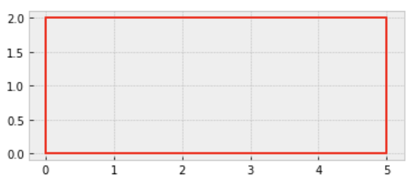
b) Write a class RightTriangle.
Include the attributes
base,height,color,perimeter,area, andvertices.Include a method
describe()that prints out the attributes of the right triangle.include a method
render()that draws the triangle on a cartesian plane.
>>> tri = RightTriangle(5,2,'blue')
>>> tri.describe()
Base: 5
Height: 2
Color: blue
Perimeter: 12.3851648071
Area: 5
Vertices: [(0,0), (5,0), (0,2)]
>>> tri.render()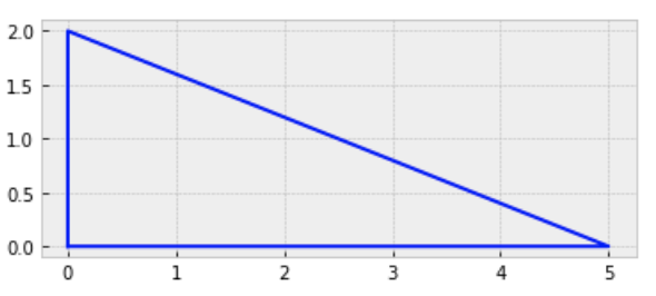
c) Write a class Square that inherits from Rectangle. Here's an example of how to implement inheritance.
Note: You should not be manually writing any methods in the Square class. The whole point of using inheritance is so that you don't have to duplicate code.
>>> sq = Square(5,'green')
>>> sq.describe()
Base: 5
Height: 5
Color: green
Perimeter: 20
Area: 25
Vertices: [(0,0), (5,0), (5,5), (0,5)]
>>> sq.render()
d) Write a class Shape with
attributes
base,height, andcolormethods
describe()andrender()
Then, rewrite your classes Rectangle and RightTriangle so that they are child classes that inherit from the parent class Shape.
The reason why we might do this is that we'd like to avoid duplicating the describe() and render() methods in each subclass. This way, you'll only have to write the these methods once, in the Shape class.
Problem 5-2
The polynomial $f(x)=x^3+x-1$ has a root on the interval $[0,1].$
a) Create a function update_bounds(bounds) that guesses a root halfway between the bounds, determines whether the guess was too high or too low, and updates the bounds accordingly.
For example, starting with the bounds $[0,1],$ the guess would be $0.5.$ This guess is too low because $f(0.5) = -0.375 < 0.$ So, the updated bounds would be $[0.5, 1].$
Now, using the bounds $[0.5,1]$, the next guess would be $0.75.$ This guess is too high because $f(0.75) = 0.171875 > 0.$ So, the updated bounds would be $[0.5, 0.75].$
Example:
>>> update_bounds([0,1])
[0.5, 1]
>>> update_bounds([0.5,1])
[0.5, 0.75]b) Create a function estimate_solution(precision) that estimates the solution to $f(x) = x^3+x-1$ by repeatedly calling update_bounds until the estimated solution is guaranteed to be within precision of the actual solution. You can start with the bounds $[0,1]$ again.
The actual solution is $0.68233 \ldots$, but this number should not appear anywhere in your code. Instead, you can find the maximum error of an estimated solution by taking half the length between the bounds.
- For example if the bounds were $[0.66, 0.7]$ then the guess would be $0.68$ and the maximum error would be $0.02.$ So, $0.68$ would be a valid output of
estimate_solution(0.1)but notestimate_solution(0.01).
Problem 5-3
Implement the following helper methods in your matrix class.
get_pivot_row(self, column_index): returns the index of the topmost row that has a nonzero entry in the desiredcolumn_indexand such that all entries left ofcolumn_indexare zero. Otherwise, if no row exists, returnNone.swap_rows(self, row_index1, row_index2): swap the row atrow_index1with the row atrow_index2.scale_row(self, row_index): divide the entire row atrow_indexby the row's first nonzero entry.clear_below(self, row_index):- Let $j$ be the column index of the first nonzero entry in the row at
row_index. - Subtract multiples of the row at
row_indexfrom the rows below, so that for any row belowrow_index, the entry at column $j$ is zero.
- Let $j$ be the column index of the first nonzero entry in the row at
clear_above(self, row_index):- Let $j$ be the column index of the first nonzero entry in the row at
row_index. - Subtract multiples of the row at
row_indexfrom the rows above, so that for any row aboverow_index, the entry at column $j$ is zero.
- Let $j$ be the column index of the first nonzero entry in the row at
Watch out!
Remember that the first row/column of a matrix has the index
0, not1.If
row1is "below"row2in a matrix, thenrow1actually has a higher index thanrow2. This is because the0index corresponds to the very top row.
Example:
>>> A = Matrix(elements = [[0, 1, 2],
[3, 6, 9],
[2, 6, 8]])
>>> A.get_pivot_row(0) (TEST ID: 1)
1
>>> A.swap_rows(0,1)
>>> A.show() (TEST ID: 2)
[3, 6, 9]
[0, 1, 2]
[2, 6, 8]
>>> A.scale_row(0)
>>> A.show() (TEST ID: 3)
[1, 2, 3]
[0, 1, 2]
[2, 6, 8]
>>> A.clear_below(0)
>>> A.show() (TEST ID: 4)
[1, 2, 3]
[0, 1, 2]
[0, 2, 2]
>>> A.get_pivot_row(1) (TEST ID: 5)
1
>>> A.scale_row(1)
>>> A.show() (TEST ID: 6)
[1, 2, 3]
[0, 1, 2]
[0, 2, 2]
>>> A.clear_below(1)
>>> A.show() (TEST ID: 7)
[1, 2, 3]
[0, 1, 2]
[0, 0, -2]
>>> A.get_pivot_row(2) (TEST ID: 8)
2
>>> A.scale_row(2)
>>> A.show() (TEST ID: 9)
[1, 2, 3]
[0, 1, 2]
[0, 0, 1]
>>> A.clear_above(2)
>>> A.show() (TEST ID: 10)
[1, 2, 0]
[0, 1, 0]
[0, 0, 1]
>>> A.clear_above(1)
>>> A.show() (TEST ID: 11)
[1, 0, 0]
[0, 1, 0]
[0, 0, 1]Problem 4-1
a) Implement a function labelEvenOdd that takes a list of numbers and labels each number as even or odd. Return a list comprehension so that the function takes up only two lines, as follows:
def labelEvenOdd(numbers):
return [<your code here>]Example:
>>> labelEvenOdd([1,2,3,5,8,11])
[(1,'odd'),(2,'even'),(3,'odd'),(5,'odd'),(8,'even'),(11,'odd')]b) Rewrite the function below so that it does not use any dictionary comprehensions. Test your function on some input to make sure it gives the same output as the function below. (Note that you may have to scroll sideways to see the full function.)
def doSomething(sentence):
return {word: sentence.replace(word, 'barnacle') for word in sentence.split(' ')}Problem 4-2
Watch this video on Big-O notation. Then, provide the Big-O notation for the following computations:
- $A+B$ where $A,B \in \mathbb{R}^{n \times n}$
- $A-B$ where $A,B \in \mathbb{R}^{n \times n}$
- $cA$ where $A \in \mathbb{R}^{n \times n}$ and $c \in \mathbb{R}$
- $AB$ where $A,B \in \mathbb{R}^{n \times n}$
- $A^n$ where $A \in \mathbb{R}^{n \times n}$ (assume the computation involves repeated matrix multiplication)
Problem 4-3
Consider the sequence defined recursively as
$a_n = a_{n-1} - 2 a_{n-2}, a_0 = 0, a_1 = 1.$
a) Write a function firstNTerms that returns a list of the first $n$ terms of the sequence: $[a_0, a_1, a_2, \ldots, a_{n}]$
>>> firstNTerms(20)
[0, 1, 1, -1, -3, -1, 5, 7, -3, -17, -11, 23, 45, -1, -91, -89, 93, 271, 85, -457]b) Watch this video on recursion. Then, write a function nthTerm that computes the $n$th term of the sequence, using recursion.
>>> nthTerm(30)
-24475Problem 4-4
a) Refactor your Matrix class so that the code is super clean.
Be sure to name your variables well. For example, you shouldn't have an attribute A.matrix -- rather, it should be A.elements.
b) In your matrix class, rewrite __init__ to take only the following parameters, all of which are optional:
shape: a tuple containing the number of rows and columns of the matrix. By default, setshapeequal toNone.fill: if a number, then set all the matrix elements equal to the value offill. However, iffillis set todiag, then set the diagonal elements equal to1and all other elements equal to0. By default,fillequal to0.elements: set the matrix elements equal to the corresponding values of the given array. By default, setelementsequal to None.
Also, include the following attributes:
shape: returns the shape of the matrix as a tupleelements: returns the matrix elements as an array
Example:
>>> A = Matrix(shape=(2,3))
>>> A.show()
[0, 0, 0]
[0, 0, 0]
>>> A.shape (TEST ID: A1)
(2,3)
>>> A.elements (TEST ID: A2)
[[0,0,0],[0,0,0]]
>>> B = Matrix(shape=(2,3),fill=1)
>>> B.show() (TEST ID: A3)
[1, 1, 1]
[1, 1, 1]
>>> C = Matrix(shape=(2,3),fill='diag')
>>> C.show() (TEST ID: A4)
[1, 0, 0]
[0, 1, 0]
>>> D = Matrix(elements=[[1,2,3],
[4,5,6]])
>>> D.show() (TEST ID: A5)
[1, 2, 3]
[4, 5, 6]c) Extend your Matrix class to overload equality and indexing.
Equality:
implement a method
isEqualthat checks if all the elements in the matrix are equal to their counterparts in another matrix.overload the equality operator (
==) using__eq__.
Indexing:
implement a method
getthat gets the matrix element at the desired index.implement a method
setthat sets the matrix element at the desired index equal to some desired value.overload the indexing operator (
[]) using__getitem__and__setitem__.- include row indexing and column indexing via the parameter
:as indicated by the example. To check if the parameterparamis equal to:, you can useisinstance(param, slice)
- include row indexing and column indexing via the parameter
Example:
>>> A = Matrix(elements = [[1, 2],
[3, 4]])
>>> A[0,1] (TEST ID: B1)
2
>>> A[0,1] = 5
>>> A[0,1] (TEST ID: B2)
5
>>> A.show()
[1, 5]
[3, 4]
>>> B = Matrix(elements = [[1, 5]
[3, 4]])
>>> A == B (TEST ID: B3)
True
>>> B[1,:] (TEST ID: B4)
[3, 4]
>>> B[:,0] (TEST ID: B5)
[1, 3]
>>> B[1,:] = [8, 9] (TEST ID: B6)
>>> B.show()
[1, 5]
[8, 9]
>>> A == B (TEST ID: B7)
FalseProblem 3-1
a) Implement a stack. That is, create a class Stack which operates on a list using the following methods:
push: add a new item on top of the stackpop: remove the top item from the stackpeek: return the top item without modifying the stack
Examples:
>>> s = Stack()
>>> s.push('a')
>>> s.push('b')
>>> s.push('c')
>>> s.show()`
['a', 'b', 'c']
>>> s.pop()
>>> s.show()
['a', 'b']
>>> s.peek()
'b'
>>> s.show()
['a', 'b']b) Implement a queue. That is, create a class Queue which operates on a list using the methods enqueue and dequeue, and peek.
enqueue: add a new item to the back of the queuedequeue: remove the item at the front of the queuepeek: return the item at the front without modifying the queue
Example:
>>> q = Queue()
>>> q.enqueue('a')
>>> q.enqueue('b')
>>> q.enqueue('c')
>>> q.show()
['c', 'b', 'a']
>>> q.dequeue()
>>> q.show()
['c', 'b']
>>> q.peek()
['b']
>>> q.show()
['c', 'b']Problem 3-2
a) Write a function makeNested which takes a "flat" dictionary and converts it into a nested dictionary based on the key names.
Example:
>>> colors = {
'animal_bumblebee': ['yellow', 'black'],
'animal_elephant': ['gray'],
'animal_fox': ['orange', 'white'],
'food_apple': ['red', 'green', 'yellow'],
'food_cheese': ['white', 'orange']
}
>>> makeNested(colors)
{
'animal': {
'bumblebee': ['yellow', 'black'],
'elephant': ['gray'],
'fox': ['orange', 'white']
},
'food': {
'apple': ['red', 'green', 'yellow'],
'cheese': ['white', 'orange']
}
}b) Write a function flatten which takes a nested dictionary and converts it into a flat dictionary based on the key names.
Example:
>>> colors = {
'animal': {
'bumblebee': ['yellow', 'black'],
'elephant': ['gray'],
'fox': ['orange', 'white']
},
'food': {
'apple': ['red', 'green', 'yellow'],
'cheese': ['white', 'orange']
}
}
>>> flatten(colors)
{
'animal_bumblebee': ['yellow', 'black'],
'animal_elephant': ['gray'],
'animal_fox': ['orange', 'white'],
'food_apple': ['red', 'green', 'yellow'],
'food_cheese': ['white', 'orange']
}Problem 3-3
In Assignment 2, you wrote a matrix class. Clean up your code for your matrix class and generalize it to $m \times n$ matrices.
Additionally,
implement the following attribute:
shapeimplement the following methods:
max,min,transpose,exponent.- Remember that to take the exponent of a matrix, you need to repeatedly multiply the matrix by itself using matrix multiplication. (Don't just exponentiate each element separately.)
overload the following operators:
+(__add__) for matrix addition,-(__sub__) for matrix subtraction,*(__mul__) for scalar multiplication,@(__matmul__) for matrix multiplication
Examples:
>>> A = Matrix([[1, 1, 0],
[2, -1, 0],
[0, 0, 3]])
>>> A.shape()
(3, 3)
>>> A.max()
3
>>> A.min()
-1
>>> A.transpose().show()
[[1, 2, 0],
[1, -1, 0],
[0, 0, 3]]
>>> A.exponent(3).show()
[[3, 3, 0],
[6, -3, 0],
[0, 0, 27]]Problem 3-4
In Assignment 1, we encountered the trivial encoding function which maps
' '$\rightarrow 0,$'a'$\rightarrow 1,$'b'$\rightarrow 2,$
and so on.
Using a linear encoding function $s(x) = 2x+3,$ the message 'a cat' can be encoded as follows:
Original message:
'a cat'Trivial encoding:
[1, 0, 3, 1, 20]Linear encoding:
[5, 3, 9, 5, 43]
a) Create a function linearEncoding(string,a,b) which encodes a string using the scrambling function $s(x) = ax+b,$
Example:
>>> linearEncoding('a cat', 2, 3)
[5, 3, 9, 5, 43]b) Decode the message
[377,
717,
71,
513,
105,
921,
581,
547,
547,
105,
377,
717,
241,
71,
105,
547,
71,
377,
547,
717,
751,
683,
785,
513,
241,
547,
751],given that it was encoded with a linear encoding function $s(x) = ax+b$ where $a,b \in \{ 0, 1, 2, \ldots, 100 \}.$
Hint: try running through all combinations of $a$ and $b,$ checking if they correspond to some decoded message, and if so, then printing out that decoded message. Then, you can visually inspect the results to find the one that makes sense.
Problem 2-1
a) Write a function intersection that computes the intersection of two tuples.
Example:
intersection( (1,2,'a','b'), (2,3,'a') )$\rightarrow$(2,'a')
b) Write a function union that computes the union of two tuples.
Example:
union( (1,2,'a','b'), (2,3,'a') )$\rightarrow$(1,2,3,'a','b')
Problem 2-2
Write a function countCharacters that counts the number of each character in a string and returns the counts in a dictionary. Lowercase and uppercase letters should not be treated differently.
Example:
countCharacters('A cat!!!')$\rightarrow${'a': 2, 'c': 1, 't': 1, ' ': 1, '!': 3}
Problem 2-3
Create a Matrix class with the methods show, add, subtract, scale, and multiply for $2 \times 2$ matrices.
The input to a Matrix object is a multi-dimensional array (i.e. an array of arrays).
Examples:
A = Matrix([[1,3],[2,4]])
A.show()
[[ 1, 3 ],
[ 2, 4 ]]
B = Matrix([[1,0],[2,-1]])
C = A.add(B)
C.show()
[[ 2, 3 ],
[ 4, 3 ]]
D = A.subtract(B)
D.show()
[[ 0, 3 ],
[ 0, 5 ]]
E = A.scale(2)
E.show()
[[ 2, 6 ],
[ 4, 8 ]]
F = A.multiply(B)
E.show()
[[ 7, -3 ],
[ 10, -4 ]]
Problem 1-1
a) Write a function letters2numbers that converts a string to a list of numbers, where space = 0, a = 1, b = 2, and so on.
Example:
letters2numbers('a cat')$\rightarrow$[1,0,3,1,20]
b) Write a function numbers2letters that converts a list of numbers to the corresponding string.
Example:
numbers2letters([1,0,3,1,20])$\rightarrow$'a cat'
Problem 1-2
Write a function isSymmetric that checks if a string reads the same forwards and backwards.
Examples:
isSymmetric('racecar')$\rightarrow$TrueisSymmetric('batman')$\rightarrow$False
Problem 1-3
a) Write a function convertToBase10 that converts a number from base-2 to base-10.
Example:
convertToBase10(10011)$\rightarrow$19because $1 \cdot 2^{4} + 0 \cdot 2^3 + 0 \cdot 2^2 + 1 \cdot 2^1 + 1 \cdot 2^0 = 19$
b) Write a function convertToBase2 that converts a number from base-10 to base-2.
Example:
convertToBase2(19)$\rightarrow$10011
Problem 1-4
Write a function isPrime that checks if a number is prime.
Examples:
isPrime(59)$\rightarrow$TrueisPrime(51)$\rightarrow$False
Hint: Check for divisibility within a for loop.